
Tech Corner: Twenty Simple Excel Tips for Financial Remedy Practitioners
Published: 13/03/2024 07:00

Microsoft Excel is a spreadsheet program for presenting formatted numbers and for performing calculations on them. It also offers basic text-editing for labelling and for explaining any figures and calculations.
The spreadsheet consists of thousands of ‘cells’. A cell may contain text, numbers, dates, formulas, calculations, or nothing. Each cell has its own format, which can be changed. Every cell is identified by its grid reference: columns (‘x-axis’) are labelled alphabetically and rows (‘y-axis’) are labelled numerically. Cells are referred to by their grid reference as A1 or G98, etc.
An Excel file is a workbook. It comprises one or many worksheets. Cells in worksheets can be linked within the workbook. A workbook can also be linked to other workbooks, but it is recommended that you avoid this as it leads to a loss of transparency, broken links if the file location is changed, the possibility of linking to unwanted (or not updated) data, and unintentional revelation to third parties of private data.
Data is entered by clicking on a cell, typing, and pressing ‘Enter’. Existing data in cells may also be edited on a PC by pressing ‘F2’ and on a Mac by typing ‘Fn + F2’ or ‘Ctrl + U’.
The tips below are specifically designed to de-mystify Excel for users who lack confidence, to explain some potentially confusing features and to provide some short-cuts. They are pitched at a basic level (advanced tutoring may follow if there is demand from FRJ readers!). There are useful keyboard shortcuts for PC and Mac users tabulated at the end of the article.
(1) Undo/redo/repeat
Crucial tools for beginners: to undo the last action type Ctrl + Z (PC) or ⌘ + Z (Mac) (⌘ is the Command button, and you don’t type the ‘plus’ sign).
To Redo (or repeat, as the context may dictate) type Ctrl + Y (PC) or ⌘ + Y (Mac).
(2) Understanding the white cross and the black cross
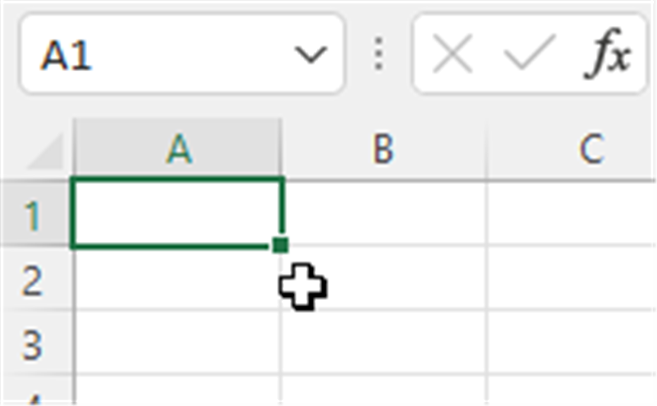
The white cross is for selecting (highlighting) cells either individually or in a group:
The black cross is the AutoFill tool, and it only appears if you hover under the bottom right-hand corner of the cell or the range of cells:
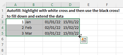
Dragging that black cross down causes this to happen:
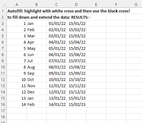
The black cross is useful for completing sequences of numbers, dates, weekdays, months, etc – play around and it is quite handy!
TIP: Make sure before you do anything that the correct cross is showing, otherwise you may get unexpected results.
(3) Knowing your left-click from your right
Left-click is generally for selection and editing. Right-click (Ctrl + click on a Mac) brings up a context-sensitive menu, the most frequently-used options being Cut, Copy, Paste, Insert, Delete and Format Cells.
(4) How to enter and check a formula
Enter a formula by typing ‘=’ in a cell. The most useful ones are SUM and simply typing mathematical operations into a cell (use +, -, * (multiply) and / (divide)). For example:
=SUM(C4:C9) will add up the contents of the six cells in the column from C4 to C9.
=0.03*500,000 will display 3% of 500,000, which is 15,000.
=G39/4 will, if G39 contains the number 800, display 200.
All formulas are ‘live’ (unless you disabled this in Formulas > Calculation Options) and automatically update if the content of any cells to which reference is made are updated.
Double-clicking a cell with a formula in it reveals any cells to which reference is made. This is useful to reveal whether any rows or cells have been omitted from a calculation.
Every cell has its own format: try to keep cells in the same row or column (depending on how you are using your data) formatted the same way.
(5) Check, and don’t over-type, your formulas
A ‘total’ box should contain a formula, summing the numbers above it. If an item’s value has changed between hearings, don’t just over-type the total, but change the value of the underlying figure (asset value, bank account balance or pension CE).
It seems that some proprietary ES2 software produces a ‘flattened’ ES2 that looks as though it contains a SUM formula, but in which the formula has in fact been removed and over-typed. This increases the likelihood of numbers appearing as though they have been correctly summed where in fact there is no calculation taking place at all! So, always check formulas are still there, and that they refer to all relevant cells above them.
(6) Format cells
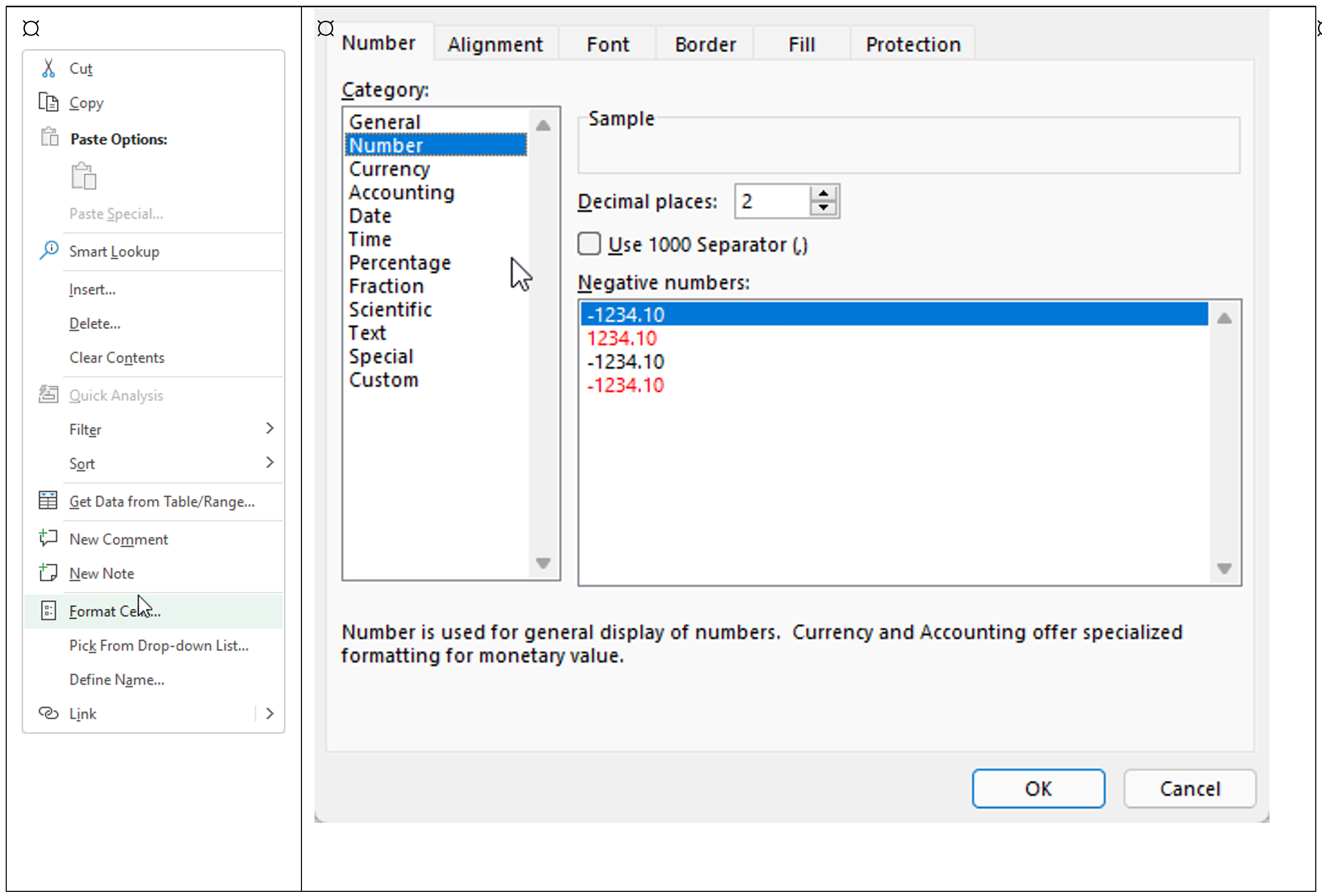
The context-sensitive menu is shown on the left below, alongside the ‘Format Cells’ multi-tabbed pop-up menu.
This is where you may adjust number and date formats, decimal places, comma-separators, borders, shading (fill) and so on (although there are short-cut icons to various commonly-used features in the main Excel screen).
NB: If you hover your mouse over an icon it gives a fuller ‘tool-tip’ as to what it does.
(7) What the ######? Changing the number of decimal places showing
Cells with too many decimal places (or even simply with ‘pence’) showing can appear as ######. Either resize the column (see below) or reduce the decimal places. To change the number of decimal places, select the relevant cell, range of cells, column or row containing the data and click on these icons:

The icon on the left is ‘Increase Decimal’ – it shows more decimal places and hence a more precise value. The icon on the right is ‘Decrease Decimal’ – it shows fewer decimal places and hence leads to the number taking up less space on the screen: this is useful if there is a lot of contention for screen-space in the spreadsheet in question!
These also work when numbers are displayed as percentages.
(8) Avoiding marching ants
If a cell is surrounded by marching ants (little dashes that move clockwise) then either press ‘Enter’ to accept the contents/calculation, or ‘Escape’ (Esc, top left) to get rid of the marching ants. This can be a reason why you are trapped in a certain ‘state’ in Excel, seemingly unable to work.
(9) Swiftly managing #REF! errors
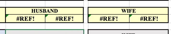
If a category of assets (e.g. chattels/other/business interests) has been deleted, then any formula referring to the deleted sub-total will display as #REF! Don’t panic, as the formula itself can be amended.
If the formula in the ‘total’ cell read ‘=F36 +F63+F70+F82+#REF!+F102’ (the #REF! referring to a deleted cell above) then amend it to say ‘=F36+F63+F70+F82+F102’. The #REF! will disappear and the correct total will be displayed. NB: Any grand total cell referring to a cell containing a #REF! would itself display #REF! until the error is fixed, and so that will be rectified upon correction, too.
(10) Fixing the formatting using Paste Special → Formats
Common errors on an ES2 are borders that are too thick/thin, or are missing, along with incorrectly shaded or inconsistently formatted cells.
For example, below, the (£4,822) has been copied from right to left along with its formatting, and so the left and centre borders have also been inadvertently changed:
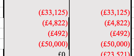
A quick fix is to select another cell, or range of cells, with the desired formatting (the cells with the (£33,125) in them, in the above example), and then Copy, and Paste Special (either via the button below or in the Edit menu):
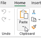
If you only want the formats of a cell or cells, then copy the cell/cells, and use Paste → Paste Special → Formats (on a Mac the shortcut in the button is ‘Keep Source Formatting’).
There are various other options. If you select ‘Paste Special’, you will see the following list of Paste options:
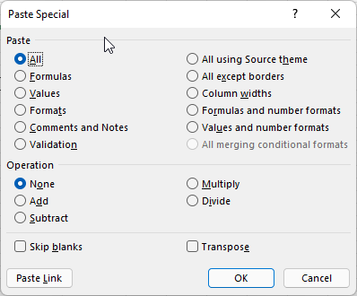
Paste Special → Values is useful for copying either the result of a calculation as if it were just a typed number, or for copying something without its formatting.
(11) Wrapping comments
‘Per H’ or ‘Per W’ in front of a comment indicates helpfully which party has asserted something which is not agreed and this enables each party to agree to the co-existence of two completing explanations in a row. Text does not ‘wrap’ (around the right-hand end of the cell) by default, but long comments should therefore be wrapped to the column width (to render the ES2 printable).
Select the cell (or the entire column if applicable to many cells), right-click (or Ctrl + Click on a Mac), Format Cells → Alignment → Wrap text (tick box). You may then need to adjust row height, as follows.
(12) Column widths and row heights
To ensure everything looks right you can adjust column widths/row heights (and then the print area too – see below):
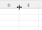
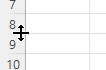
Hover over the join between two columns or between two rows and you can drag column widths or row heights.
If you hover over the join and double-click the mouse, then you will find that the column (or row, if wrapping is enabled) will jump to the width or height appropriate to the widest entry in the column. Be careful with this, as sometimes that is not what you in fact want (Excel allows cell contents to cover adjacent empty cells, and so this is not always necessary).
NB: Whilst it is possible to ‘Hide’ columns or rows: in my experience this creates all sorts of opportunities for leaving old data kicking around in a re-used spreadsheet, or sub-totals that feed in to totals but are invisible. Hiding columns should therefore be avoided pretty much always as it is too dangerous.
(13) Dealing with hidden columns/rows
You will know that there are hidden rows or columns if row/column numbers are not continuous.
Unhide columns by selecting columns either side of the hidden column, right-clicking and then selecting ‘Column Width’ from the pop-up menu (similarly with ‘rows’ and ‘Row Height’).
Setting Column Width to something like 12 will reveal it, and then you can drag the width as above.
(14) Inserting and deleting
To delete the contents of a cell, click on it and press the backspace or delete keys. It becomes a blank cell, but nothing around it changes.
To delete an entire row or column: first select it by clicking on the row or column header. In the pop-up menu that appears upon right-click (PC) or Ctrl + Click (Mac), select ‘Delete’. If you selected a range of cells (this can lead to unintended results …) then you will be asked what you want to happen to the cells around it. You can mercifully swiftly undo any poor-decision making here.
To insert a number of rows then select the entire row (and as many rows below as you intend to insert) before which your new row is to be inserted and from the right-click/Ctrl + click pop-up menu select ‘Insert’. New rows appear whose cells inherit the formatting of the cells in the row above the row you inserted.
(15) Selecting large parts of a worksheet – do it in reverse
Find the bottom right cell in your worksheet and then select backwards with the white cross, moving top-left, towards cell A1. This prevents you accidentally selecting (if moving towards the bottom right) hundreds of thousands of blank cells.
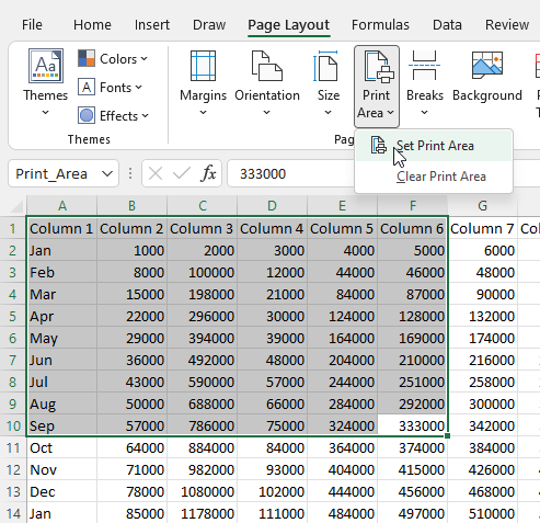
(16) Setting the print area
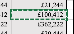
To print only a certain part of the page, go to Page Layout → Print Area → Set Print Area
In the example below, only columns A–F and rows 1–10 will print:
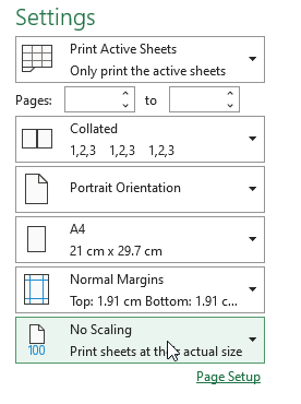
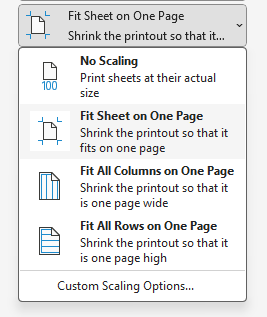
(17) Making your print-outs fit onto one page
It is frustrating to have most of the information on one page, and then the final column on its own on an adjacent page. To solve this, you can instruct Excel to fit the entire sheet (meaning the print area) or all columns/all rows onto one page. The option to do so is found in the Print menu under Settings on the left-hand-side:
(18) Repeating rows at the top of each printed page
It is possible to repeat certain rows (e.g. those containing column headings) at the top of each printed page. To set this up, in ‘Normal’ view go to Page Layout → Print Titles:
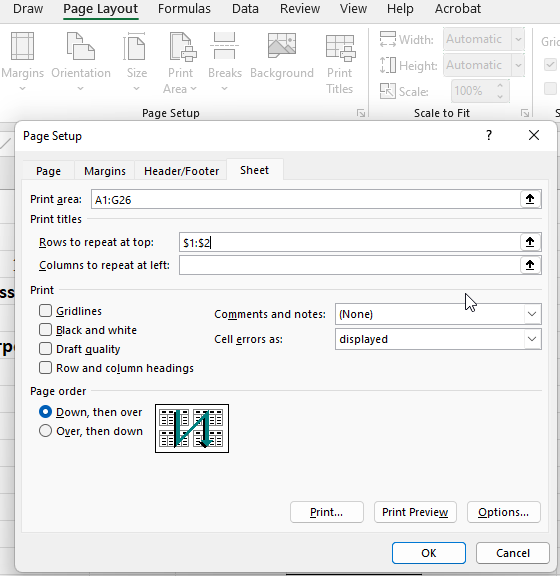
The settings above will repeat the contents of rows 1 and 2 on each printed page.
(19) Single quotation marks to control how Excel treats your data
If text or numbers you enter are not displaying correctly because Excel is auto-detecting a format (e.g. where the last four digits of a bank account number start with a zero, or where you wish to use only the month and year of a date and Excel insists on adding the day), then typing a single quotation mark before the text will make Excel render everything you type in that cell as text.
(20) Aligning text and fixing text that won’t align
You can make text or numbers in cells align left, right, centre or top and bottom using the following (self-explanatory) icons on the ‘Home’ menu:
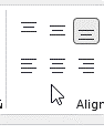
NB: Ignore the ‘Decrease Indent’ and ‘Increase Indent’ icons that are next to these, as they are not particularly useful in Excel.
If, following this, your comments are all supposed to be correctly aligned but the text is still indented in certain entries, then select the entire (text) column (or relevant misbehaving cells only) and change the format using Format Cells → Number → Category to ‘Text’.
Some useful keyboard shortcuts
| PC | Mac | Operation |
| Ctrl + W | ⌘+ W | Close workbook |
| Ctrl + O | ⌘+ O | Open a workbook |
| Ctrl + S | ⌘+ S | Save workbook |
| Ctrl + X | ⌘+ X | Cut text/cell(s) |
| Ctrl + C | ⌘+ C | Copy text/cell(s) |
| Ctrl + V | ⌘+ V | Paste text/cell(s) |
| Ctrl + Alt + V | Opt + ⌘+ V or Ctrl + ⌘+ V | Paste Special (menu) |
| F5 | Fn + F5 | Go to a specific cell (e.g. F8/A7) |
| F2 | Ctrl + U, Fn + F2 | Edit contents of a cell (either in the cell itself or at the top of the worksheet |
| F4 | ⌘+ T | Absolute Reference toggle |
| Ctrl + Home | Ctrl + Fn + Left Arrow | Jumps to top left (cell A1) |
| Ctrl + End | Ctrl + Fn + Right Arrow | Jumps to bottom right |
| Ctrl + B | ⌘+ B | Bold |
| Ctrl + I | ⌘+ I | Italic |
| Ctrl + F | ⌘+ F | Find something |
| Ctrl + H | Ctrl + H | Replace something |
| Ctrl + Z | ⌘+ Z | Undo |
| Ctrl + Y | ⌘+ Y | Redo something you just undid OR Repeat something you have just done |
| Ctrl + [ | CTRL + [ | Goes to cell or cells referred to in the calculation in the cell you are in! |
| Ctrl + ] | CTRL + ] | Goes back to the cell you started in |
| Alt + | (No direct equivalent) | Adds up the column above the cell you are in using SUM |
| Ctrl + F6 | (No direct equivalent) | Cycles between workbooks |
| Ctrl+Pg Up/Pg Dn | CTRL + Fn + Up Arrow/Down Arrow | Moves between worksheets in a workbook |
 ©2024 Class Legal classlegal.com