Report of the Duxbury Working Party (provisional), September 2024
Published: 02/10/2024 13:31
- Michael AllumMichael Allum is a Solicitor and Partner at The International Family Law Group LLP. He specialises in finance cases with a particular emphasis on matters with an international element. He is also regularly instructed on cases regarding financial provision after an overseas divorce (Part III). He is a member of the Financial Remedies Journal editorial board and of the Duxbury Working Party.
- Simon Bruce
Simon is a solicitor and Partner at Dawson Cornwell LLP. He is also a pro bono lawyer at law clinics in London. Simon has practised for over 41 years. He is a member of the Duxbury Working Party and writes the ‘Thought Leader’ in Family Law. He comes from Lancashire.
- Sarah Hoskinson
With over 20 years’ experience in complex financial remedy cases, Sarah is a Partner and Head of Burges Salmon’s Family & Divorce practice. She sits on a number of financial remedy and other technical groups, including the Family Justice Council Financial Remedy Working Party, FJC Working Party on Needs, the Pension Advisory Group (PAG and PAG2) and the IAFL Pensions Committee, which she chairs. She is also a member of the Duxbury Working Party.
- Lewis Marks KCLewis Marks QC is a family law barrister at QEB, specialising in financial remedy cases. He has been an editor of At A Glance since 1999, and is also a founder editor of the Financial Remedies Practice. He was an original member of the Duxbury Working Party in 1998 and has authored a number of papers on the subject of Duxbury calculations. He has acted as Chair and convenor of the reconstituted Duxbury Working Party.
- Sir Nicholas MostynSir Nicholas Mostyn was a judge of the High Court, Family Division, and of the Court of Protection 2010–2023. He was a founder editor of At A Glance and of Financial Remedies Practice and continues as editor-in-chief of both publications. He is a member of the Duxbury Working Party.
- Joe RainerJoe is a junior barrister at QEB. He has a specialist matrimonial practice, with a focus on financial remedies and cases brought under TLATA 1996. He has appeared in several well-known reported cases and writes and lectures frequently on a variety of topics. He is a member of the Financial Remedies Journal editorial board, an editor of At A Glance, and a co-author of the fourth edition of Pensions On Divorce: A Practitioner’s Handbook. He is also a member of the Pension Advisory Group and the Duxbury Working Party.
- Mary WaringMary is a chartered financial planner, chartered accountant and Resolution Accredited Specialist. She is the founder of Wealth for Women, an award-winning company specialising in financial advice to women going through divorce. She is a member of the Duxbury Working Party.


Provisional report: This report has been prepared without any prior public consultation. It is published provisionally to allow interested parties to respond. Responses should be emailed to j.rainer@qeb.co.uk by 1 November 2024 and will be considered by the Working Party ahead of publication of our final report which we intend will be on 15 November 2024.
Executive summary
1. Duxbury calculations, whether presented as a printed table or by specialist software, have for nearly four decades been the tool of choice in the family courts for the assessment of lump sums necessary fairly to provide for a clean break in a case where there would otherwise have been a periodical payments order.
2. The underlying assumptions have been the subject of criticism in articles in legal journals, generally on the basis that the sums arrived at are not sufficient to provide the level of spending power intended for the lifetime of the recipient.
3. Those underlying assumptions have not been the subject of any general review for many years. This report is by an ad hoc and self-selected group of interested professionals to undertake that review, including, in the light of the criticisms, the methodology. The Working Party has no status to make any decisions about how the courts should approach Duxbury calculations. It proffers the proposals in this report to banish outdated concepts and generally to modernise the approach. It will be a matter for the courts whether to adopt the recommendations.
4. Our main conclusions are, in summary:
4.1. The existing underlying assumptions as to income yield (3%), capital growth (3.75%) and inflation (3%), remain essentially sound.
4.2. The calculation should also include an allowance for the management charges (1% for funds up to £1m, 0.5% for funds above £1m) likely to be suffered on the investment of the fund.
4.3. The calculation should no longer default to the life expectancy of the recipient (although there will be cases in which that is appropriate), rather the court should consider the likely duration of the periodical payments order which is being capitalised, and apply that period to the quantum of the periodical payments that is being capitalised.
4.4. The computation should not default to the inclusion of the State Pension, although the fact of such entitlement may impact on the quantum of the periodical payments being capitalised.
4.5. It is neither necessary nor appropriate (where the appropriate duration for the calculation is a term of years and as State Pension age is now the same for men and women) to have separate tables for male and female recipients.
4.6. Where whole-of-life is determined to be the appropriate duration for the calculation extreme caution should be exercised in undertaking a Duxbury calculation for any payee whose life expectancy is less than about 15 years, although we think that these will be very rare cases.
4.7. Legal advisers to parties who are receiving Duxbury based awards, or awards with a Duxbury component, should ensure that their clients have a proper understanding of the basis of the calculation and disabuse them of the erroneous belief that it ensures a particular level of expenditure for a particular period.
5. While our recommendations in relation to management charges and State Pension will tend to increase awards, we anticipate that in practice this will be mitigated, and sometimes outweighed, by the adoption of our recommendation for a lesser duration than life expectancy in most cases.
Terminology
6. In this report we use the following terms:
6.1. ‘Financial remedy’ to encompass all financial awards made by agreement or court adjudication following relationship breakdown (generally divorce, but including dissolution of a civil partnership), notwithstanding that much of the jurisprudence deploys now antiquated terminology such as ancillary relief.
6.2. ‘Periodical payments’ for what is sometimes referred to as maintenance or alimony, being regular payments made to another person (usually a spouse, ex-spouse or co-parent) as a financial remedy.
6.3. ‘Joint lives’ to mean an award of periodical payments with no term specified which endures until the death of either party unless varied or discharged by a subsequent order, or until the remarriage of the payee.
6.4. ‘Payee’ to mean the recipient of a financial remedy award.
6.5. ‘Payer’ to mean the party against whom a financial remedy award is made.
Background
7. The Duxbury calculation originates from the work of accountant Tim Lawrence then of Coopers & Lybrand, instructed as an expert witness on behalf of Mrs Duxbury during the course of her financial remedy proceedings consequent upon the breakdown of her marriage to Mr Duxbury in 1984.
8. Mr Lawrence had devised a spreadsheet which worked out by trial and error the lump sum which in his opinion might fairly enable Mrs Duxbury to meet her ‘needs’ pursuant to the then newly implemented obligation imposed on the court to achieve a clean break. The calculation was of the capital payment in the form of a lump sum (a ‘Duxbury fund’) which, if depleted at a steady rate in real (inflation adjusted) terms, allowing for assumed income yield and capital growth while invested, and allowing for the depredations of tax on income and on realised capital gains, would theoretically be exhausted on the date of Mrs Duxbury’s actuarially anticipated death. Lord Nicholls of Birkenhead gave a graphic description of the concept in White v White [2000] UKHL 54 at [39]: ‘The Duxbury fund calculation involves using income and ultimately exhausting the capital at the theoretical point when the wife would down her last glass of champagne and expire as predicted by the life tables.’
9. Mr Lawrence’s modelling was accepted by the court (Reeve J at first instance, and a Court of Appeal comprising Ackner, Stephen Brown and Parker LJJ). Although the judgment of the Court of Appeal was given in November 1985, it was not reported until 1987 (Duxbury v Duxbury [1987] 1 FLR 7) and the report itself says nothing about this method of calculation. However, the existence of Mr Lawrence’s calculation became known, and the thoughts of professionals turned to creating, in what was then the relatively new medium of the spreadsheet,1 an iterative program which would work out the discounted lump sum payment to be made in lieu of what would otherwise be a series of periodical payments. Nicholas Mostyn believes he wrote the first such program in 1989.2 Other such programs followed.
10. The program asked the user to input the claimant’s annual spending requirement and age and then made a ‘guess’ as to the required capital sum, with the calculation being conducted repeatedly (iteratively), refining the ‘guess’, until the remaining figure at the terminal date was zero.
11. The arithmetic involved a number of ‘assumptions’ including that:
11.1. The claimant, Mrs Duxbury, would die on, and neither before nor after, her actuarially estimated date of death, but without regard to any individual characteristics that she might have which would tend to either shorten or lengthen her life as compared to her standardised or actuarial life expectancy based solely on her date of birth.
11.2. Inflation would remain at a constant level throughout the period of her life.
11.3. The income yield (‘yield’) would remain at a constant level throughout her life.
11.4. The gross capital appreciation (‘growth’) of her investments would remain at a constant level throughout her life.
11.5. Taxation of both income and gains would be met from the fund, with only the allowances and bands altering (in line with the assumed constant rate of inflation), and without Mrs Duxbury or her advisers taking any steps to invest in ways which would reduce that tax burden.
11.6. The claimant would be entitled to a full State Pension at the then applicable commencement date.
11.7. Income would be spent first, then capital drawn as required, including the relevant proportion of gains comprised in the capital (attracting tax where applicable) but also – and initially largely – the original capital (which would be tax free). The proportion of gains would increase as the original capital was gradually depleted.
11.8. Additional realisations would take place annually, equal to a fixed percentage (3%) of the remaining funds, for reasons of proper management of the fund and/or because of market forces requiring such realisations (this was called ‘churn’), which might also give rise to a liability to tax to be paid as it arose.
11.9. No consideration was given to the possibility that the claimant might remarry – indeed, Mr Duxbury’s appeal against the order on the basis that this possibility should have been factored in to reduce the award was dismissed by the Court of Appeal.
12. The calculation was not wholly unlike a discounted cash flow model, or the kind of computations then used to calculate lump sum awards in personal injury or medical negligence cases, which generally operated on the basis of a ‘discount’ for the advance payment of a fixed sum to be depleted over a period of years.
13. For a few years an industry arose where accountants would be instructed in individual cases to put forward bespoke computations adopting some or all of the assumptions put forward by Mr Lawrence, supplemented with their own variations, particularly as to investment yield, capital growth and inflation (to which we shall refer as the ‘key assumptions’), but sometimes also in relation to life expectancy. It soon became apparent that costs, common sense and appropriate allocation of court resources favoured a standardisation of the arithmetic and ‘assumptions’ rather than evidence being given, submissions being made, and judgments delivered in every case.
14. By 1991 the concept of a Duxbury calculation had received judicial endorsement. In B v B [1990] 1 FLR 20 Ward J said ‘if this calculation is accepted as no more than a tool for the judge’s use, then it is a very valuable help to him [sic] in many cases’. in Gojkovic v Gojkovic [1990] 3 WLR 261 Butler-Sloss LJ stated that ‘a Duxbury calculation … produces a figure to which the judge is entitled to have regard in deciding what is the right answer’.
15. In 1991 a group comprising Nicholas Mostyn, Peter Singer QC, James Holman QC and Valentine Le Grice worked on the production of the first edition of the Family Law Bar Association’s flagship annual publication At A Glance, which came out in 1992. It was decided that it should contain a table giving guideline Duxbury figures based on just two variables: the age of the payee (specifically, until 2001/02 only for women3) and the target amount of the revenue ‘need’ in the first and all subsequent years. From inception to date those tables have proceeded on a ‘whole life’ basis – i.e. that the inflation adjusted spending requirement would continue for the remaining actuarial life expectancy of the recipient.
16. This table was updated annually to reflect changes in life expectancies (as predicted by the Government Actuary and the Office for National Statistics) and changes in the applicable rates of tax, including future changes which had been announced even if not yet implemented. There also became available commercial software to undertake ever more bespoke computations,4 most notably and popularly, Capitalise by Class Legal, first produced in 2000.
17. The aggregation of the key assumptions gives a real rate of return (RRR): income yield + capital growth – inflation = RRR. That was initially set at 5%. In ‘Reflections on Duxbury’ in the 1995 edition of At A Glance the editors stated:
‘In the introductory material to Actuarial Tables for use In Personal Injury and Fatal Accident Cases (HMSO, 2nd edition 1984) the Ogden Committee point out that for a payee to be certain to receive an inflation-proof income for the period to which the loss relates it would be necessary to invest in Index-Linked Government Stock. The return upon these has historically ranged between 2.5% and 4.5% gross. The rate applicable on 30 January 1995 was 3.89% before tax (source: Financial Times). By contrast the gross real return on equities has over the 25 years to 1993 averaged 5.8% (source: The BZW Equity-Gilt Study Investment in the London Stock Market since 1918). …
The lower the percentage real rate of return selected, the higher the capital fund required. So the choice made for these Duxbury tables of 4.25% should be regarded as fair to each spouse, and designed to cover such considerations as any professional expense in managing the award, once made.
Whereas therefore the previous editions of At A Glance have suggested that it was a matter for evidence and argument in each case what assumptions should be adopted, it may now be that such a laissez-faire approach is outmoded. It would be better to accept that (for the illustrative purpose which is all that the calculation can provide) an industry-standard of 4.25% should be adopted as the real rate of return in current and foreseeable financial circumstances.’
18. This was followed by F v F (Duxbury Calculation: Rate of Return) [1996] 1 FLR 833 where Holman J stated:
‘Although I am a member of the editorial committee of At A Glance (FLBA) I was not the author of “Reflections on Duxbury” to be found at the beginning of the 1995 edition. But I agree with its reasoning and its conclusions. In my view it is important that there should indeed be “an industry standard” for the purpose of the Duxbury approach and in my experience that standard has already settled at around 4.25%’
19. In 1998 the original Duxbury Working Party came into existence. It was a self-selected group of (male) lawyers, accountants and actuaries who shared an interest in the topic and had sufficient understanding of both the underlying object of the calculation and the workings of it, as well (at least for some members) the expertise to identify appropriate figures for the key assumptions. They had no status or standing other than their willingness to discuss and publish the outcome of their discussions in the commentary to the annually updated Duxbury table published in At A Glance. It produced its first report quickly ‘Duxbury – The Future’: [1998] Fam Law 741 proposing a RRR of 4.25%. Unsurprisingly, that was adopted by the editors of At A Glance. From 1998 until 2006 there were occasional, but by no means annual, adjustments made to the key assumptions, in line with the collective or majority views of the then members of the original Duxbury Working Party, of which the authors of this report are a reconstitution.5
20. In practice the adjustments, if any, tended to be de minimis, since the view of all members of the Working Party was that even seemingly dramatic events in the financial landscape (for example Black Monday in 1992 when the FTSE 100 fell by over 11% in a single day, while the Dow Jones fell 20%) would usually be ‘blips’ in an otherwise historically clearly identifiable trend. Views about what had happened in the last 15 months were not determinative when considering an investment horizon measured in many decades.
21. In January 2002, the Duxbury Working Party reconvened and recommended that from April 2002 calculations should be done using a RRR of 3.75%. This led to two tables being published in the 2002–2003 edition of At A Glance one using a RRR of 4.25%, the other a RRR of 3.75%. That rate of 3.75% was approved by the court in GW v RW [2003] EWHC 611 (Fam), [2003] 2 FLR 108 at [57] where N Mostyn QC stated:
‘It might seem hubristic of me to approve in my capacity as a deputy High Court judge a rate recommended by me (among others) in my capacity as a member of the working party. But it is blindingly obvious that as between 4.25% and 3.75%, the lower figure is right. Indeed, present market conditions might suggest that 3.75% is distinctly optimistic. If by making this statement I can help to avoid some needless controversy about rates of return in some future case then I consider it will have been justified.’
22. In the 2009–2010 edition it was explained that the assumed income yields for years 1 and 2 had been reduced in the light of the global financial crisis and that the advice of the Duxbury Working Party was awaited. The Duxbury Working Party duly met again in 2009 and recommended a reduction in the assumed income yield in the first year to 1.5% which was adopted, and which remains in place.
23. These minor variants aside the key assumptions (income yield 3%, capital growth 3.75%, inflation 3%) have remained essentially undisturbed since the 2003–2004 edition (20 annual editions). In 2015, they received detailed judicial consideration and approbation in JL v SL (No 3) [2015] EWHC 555 (Fam) which also approved the underling algorithmic architecture. While it has always been open to individual litigants to argue against the adoption of the standard assumptions, in practice it would require a good argument or an unusual factual scenario for such an argument to succeed. There is, so far as we can tell, no recent authority in which such arguments have been successful.
24. That the calculation – and the assumptions underpinning it – were only a ‘guide’ or ‘tool’ and not ‘the rule’ in any particular case was repeatedly emphasised in the authorities, although inevitably, deviations from the guide were the exception rather than the norm. Generally, where the court was persuaded to make an order on a basis different from the result thrown up by a Duxbury calculation, the order was more generous to the claimant. That has not been because of a departure from the assumptions, but because of the specific factual matrix against which the calculation was being utilised.
25. A table giving the key assumptions and the RRR in each annual edition of At A Glance is at Appendix 2.
Criticisms
26. The Duxbury calculation – but in particular the key assumptions deployed in it – have been the subject of criticism by practitioners, financial advisers and academics alike in articles appearing in both legal and academic journals. A list of the articles which we have considered appears in Appendix 3.
27. Most of those criticisms centre around the unlikelihood, in reality, of a recipient of a Duxbury fund as an element of their financial remedy award, actually being able to invest their fund so as to enable them confidently to spend at the rate assumed as the starting point of the computation of the capital sum, without risking running out of money during their life. The common theme of the criticisms was, directly or indirectly, that the calculation was unduly mean and that claimants were being short-changed.
28. Amongst the objections have been that:
28.1. there is no protection for the payee if they turn out to be long-lived and therefore potentially surviving beyond the exhaustion of their fund even if it had otherwise performed as anticipated in the calculation,
28.2. the investment returns assumed could only be achieved (if at all) with a relatively risky investment strategy, and
28.3. the payees are likely to be more cautious than adventurous investors, and would generally not be financially sophisticated.
29. This has been argued, in effect, to place unfair risk on the payees – predominantly women – for the benefit of the payers – predominantly men. The payees were left, according to the critics, faced with either reducing their expenditure immediately or later in life when the funds were likely to be dwindling, or hoping to remarry, rather than being able confidently to continue with the lifestyle judged to be appropriate at the time of the establishing of the quantum of their Duxbury fund.
30. Defenders of the status quo focussed not so much on the likelihood that in practice the fund could be prudently invested so as to enable spending to continue at the initially assumed rate, but rather on the balance of fairness between divorcing spouses and the true aim of the calculation being to establish the fair sum to be paid immediately to compensate the payee for forgoing what would otherwise be their right to receive maintenance by way of periodical payments.
31. This has been explained in the text accompanying the Duxbury Tables since the 2010–2011 edition. In that edition it was stated:
‘… the assumptions must be such as strive to achieve fairness between the parties. An ancillary relief award is a “nil gain sum” – so any benefit to one party is necessarily a detriment to the other. The capitalisation of a periodical payments award should therefore aim to achieve as fair a balance as possible between ensuring that the payer does not pay too much and that the payee receives enough but no less. Standardisation inevitably leads to anomalies and occasionally unfair results in individual cases. A payee who capitalises her periodical payments for a lump sum calculated on Duxbury assumptions is a net winner if she soon remarries (or cohabits in circumstances which would have led to a reduction in her periodical payments) or, more paradoxically, if she dies young. On the other hand, she will be a net loser if she lives singly for longer than her average contemporary. The likelihood of re-marriage by the payee, or a payer’s inability to continue to make periodical payments long into old age, are factors which would tend to favour the recipient.’
32. In the 2024–2025 edition the explanation was put this way:
‘The calculation is not, and never has been, to work out the sum which is the equivalent of a guaranteed index-linked annuity for the life of the recipient.
Rather, it is an attempt to identify a fair net present value of a periodical payments award (where the applicant’s right to claim under the Inheritance (Provision for Family and Dependants) Act 1975 remains open) i.e. a maintenance award that endures until the death of the claimant.
The latter is likely to be materially less than the former for many reasons including the variability of a periodical payments order and its automatic cessation on remarriage.’
33. This reconstituted Duxbury Working Party has been established to consider and discuss the competing arguments and to make recommendations for the retention or adjustment of any of the underlying assumptions, but particularly those identified as the ‘key assumptions’.
34. In the course of discussion all of the members expressed disquiet about the implicit steer towards ‘whole-of-life’ provision in the Duxbury calculation by the publication of tables which provide a ‘guide’ as to the sum targeted at the actuarial life expectancy of the payee, which runs counter to the modern practice of achieving financial independence rather than lifelong dependence following marital breakdown, and counter to the statutory directive to consider financial provision by way of periodical payments ‘only for such term as would … enable the party in whose favour the order is made to adjust without undue hardship to the termination of his or her financial dependence on the other party’.6 While that provision does not apply directly to lump sum payments if, as discussed below, the proper rationale for the Duxbury calculation is of the fair sum to pay in compensation for not receiving a periodical payments order, it appears to us to be illogical, if not irrational, to assume in that calculation that the periodical payments would endure for the whole of the payee’s life.
35. The members now7 comprise five men and two women, two barristers, three solicitors, a chartered financial planner and one retired High Court Judge.
The legal framework
36. Prior to 1984 the family courts were enjoined to exercise their powers under Part II Matrimonial Causes Act 1973 so as to put the parties, as near as was practicable, in the position in which they would have been had the marriage not broken down – the so-called ‘minimal loss objective’.
37. The ‘usual’ order was provision for a home and for maintenance by way of periodical payments. Periodical payments were, and still are, always susceptible to variation (in either direction) including termination. Such payments are automatically terminated by remarriage of the payee. However, before 1984 such periodical payments orders were often, even usually, expressed as being ‘during joint lives’.
38. Such an order would end automatically on the death of the payee and, unless secured, also on the death of the payer – although recourse might then be had in an appropriate case to an application under the Inheritance (Provision for Family and Dependants) Act 1975 to obtain relief against the deceased’s estate, so long as the payer had died domiciled in England or Wales.
39. A periodical payments order might also be made for a limited period (a ‘term’ order). In the absence of a specific bar (under s 28(1A) Matrimonial Causes Act 1973 introduced in 1984) the payee could apply for such a term to be extended (under s 31).
40. But also newly introduced in October 1984 was what has become to be understood as the prioritisation of the clean break. Sections 25A and 31(7) Matrimonial Causes Act 1973, both inserted in 1984, required the court when considering an application for the first time (s 25A) or for variation of an existing periodical payments order (s 31) to ‘consider whether it would be appropriate’ to exercise its powers8 so as to bring about a clean break ‘without undue hardship’ to the claimant.
41. Duxbury (heard at first instance and on appeal in 1985) was one of the earliest cases in which the court considered how fairly to arrive at a figure for a lump sum in place of what would previously have been periodical payments, and usually on ‘joint lives’ terms, albeit supposedly in the shadow of the then new s 25A.
42. Mr Duxbury appealed to the Court of Appeal against the making of such an award having regard to the fact that Mrs Duxbury was, and had been at the time of the hearing at first instance, cohabiting with another man and was, he argued, likely to remarry. His appeal was dismissed, the Court of Appeal considering that her cohabitation was ‘irrelevant’.9
43. This is the context in which the computation of the Duxbury lump sum figure has to be viewed. It is in substitution for a stream of periodical payments with all of the variability and uncertainty that come with such a stream. The lump sum payment serves to liberate both the payee and the payer from the continuing financial interconnection of a periodical payments order but should in other respects be financially neutral for them both. That this is the essential premise of the calculation has been made clear in 13 consecutive editions of At A Glance since 2010–2011.10
44. Between 1987 and 2000, the Duxbury calculation dominated the computation of awards in cases in which a clean break was plausibly achievable. Thus, in Harris v Harris [2001] 1 FCR 68 Thorpe LJ observed that the table had an ‘obvious utility’ offering the judge a starting point. But, in reality only a very small proportion of separating couples had anything like the resources necessary to enable a Duxbury calculation to be relevant to the computation of an award – this was essentially the province of the wealthy and the comfortable professional classes. It required the parties to have available to them sufficient capital to provide homes for them both and have sufficient surplus capital to render the capitalisation of any needs-based revenue claim feasible.
45. The legal landscape in that period meant that in moderately large and very large money finance cases, the applicant’s award was usually computed as the sum of their housing requirement (usually the purchase price and ancillary expenses) and the sum necessary to compensate for the clean break imposed by reason of s 25A and the dismissal of what would otherwise have been their claim to periodical payments (as mentioned, at that time, frequently on a joint lives basis).
46. That all changed in October 2000 when the House of Lords in the case of White v White [2000] UKHL 54, ruled that the general rule should be that the ancillary relief award should be measured against the ‘yardstick of equality’. That in turn led in 2006 to the identification by the Supreme Court, in Miller v Miller; McFarlane v McFarlane [2006] UKHL 24, [2006] 2 AC 618 of the ‘sharing principle’.
47. In larger cases, in which there were significant capital assets to be divided, ‘needs’ – usually characterised as ‘reasonable requirements’ – no longer provided a limit to the quantum of claims against the wealthier spouse’s resources. Duxbury was to a large extent relegated to cases in which – for whatever reason – the sharing principle was not engaged. Examples of cases in which the sharing principle was less likely to curtail the relevance of needs/periodical payments and therefore Duxbury calculations were those in which:
47.1. the overall wealth was largely non-matrimonial having been inherited or brought into the marriage by one spouse (e.g. from a previous marriage or a pre-existing business);
47.2. the capital claims had already been dealt with and the current application was for the capitalisation of an existing periodical payments award; or
47.3. (after 2010 and the decision of the Supreme Court in Radmacher v Granatino [2010] UKSC 42) there was a prenuptial or postnuptial agreement to which effect was to be given, under which the sharing principle had been disapplied by agreement, but which left the needs of the claimant spouse at large.
48. Duxbury calculations were also frequently carried out in sharing cases as a means of cross-checking whether an applicant’s sharing award would meet their needs in moderately large to large money cases. The common practice, which remains in place today, is to identify the appropriate portion of an award necessary to meet an applicant’s capital need (often housing), and then use Duxbury, or a bespoke calculation adopting the Duxbury assumptions, to check whether the remainder of the award is sufficient to meet the applicant’s income need. This analysis sometimes precipitates argument about the fair assumptions to be adopted in the bespoke Duxbury calculation – most often when, and the extent to which, an applicant should be expected to amortise their ‘free’ capital fund to meet their annual income needs in circumstances where the other party is able to better preserve their capital share by meeting their needs from earned income.
49. The Court of Appeal has declined to endorse a default approach and considers that it is a fact specific evaluation to be carried out in each case (Waggott v Waggott [2018] EWCA Civ 727). In contrast, in CB v KB [2019] EWFC 78 at [53] Mostyn J was in no doubt that a recipient of a Duxbury fund should almost invariably be expected to amortise it.11 Of course, a conventional Duxbury calculation presumes complete amortisation of the capital fund.
50. Another trend in the law, or at least in the application of the law, over the period from 1985 to the present day, has been the almost total disappearance of the previously ubiquitous ‘joint lives’ periodical payments order. While such orders are still made from time to time, they are of increasing rarity.12 This has been a consequence of a combination of socio-economic and legal developments. The strengthened status of women in the workplace, the increased proportion of women, but in particular mothers, who continue in employment after marriage and the increasing expectation that even those who do not stay in employment remain potentially employable following a divorce, no doubt all played into the decline in joint lives order. On the legal side it was the combination of the greater embracing by the court of the desirability of the clean break, the introduction of pension sharing as well as the sharing principle, which have all contributed to the near extinction of the ‘joint lives’ periodical payments order. This is exemplified by the decision in SS v NS (Spousal Maintenance) [2014] EWHC 4183 (Fam),13 following which joint lives maintenance orders have become an endangered species, and secured joint lives periodical payments for a claimant in middle-age virtually extinct.
51. One potentially significant reason for the decline in the making of joint lives periodical payments orders is, of course, the availability of the power to make a lump sum order, typically quantified on the basis of a Duxbury calculation. However, even allowing for this the advent of the pension sharing order (with effect from 1 December 2000) would surely have greatly reduced the number of cases in which periodical payments would ever be ordered to continue beyond the normal retirement age of the payer.
52. Nonetheless, the published Duxbury methodology has continued to provide figures – at least in the print versions – exclusively on the basis of a whole-of-life entitlement of the payee, by fixing the duration of the dependency to be capitalised to the actuarial life expectancy of the payee. This might be thought to be of marginal relevance in the general run of cases and to cater only for a minority clique.
53. That is the background against which the Working Party has focussed its discussions leading to the recommendations in this provisional report.
The issues
54. Central to the discussions amongst the members of the Working Party have been the following questions:
54.1. What is – and what should be – the proper rationale and basis of a Duxbury calculation?
54.2. Is the overall algorithmic model apt or inapt for such calculations?
54.3. If inapt, what recommendations might we make for its replacement?
54.4. What is a realistic long-term average rate to assume for inflation, or otherwise factor into the calculation?
54.5. What are realistic income yield and capital returns to assume on an investment portfolio representing a Duxbury award to achieve the appropriate objectives?
54.6. How, in answering that question and if at all, should fund management costs be taken into consideration and at what stage?
54.7. Should the courts be encouraged or discouraged from abandoning reliance on published tables and seeking bespoke evidence in individual cases?
54.8. Should the individual characteristics and proclivities of the payee be taken into account in such an exercise (for example real or claimed reluctance to take investment risk, or considerations of familial longevity or the opposite)?
54.9. Does the practice of publishing tables of Duxbury figures based only on ‘whole-of-life’ provision lead to a disproportionate number of awards or settlements being based on the false premise that the alternative would have been a ‘joint lives’ order?
54.10. With what ‘health warnings’ should Duxbury calculations be endorsed better to educate both lawyers and, more importantly, lay parties about the differences between such a fund and a guaranteed income for life as if from an annuity?
The rationale for a Duxbury calculation
55. Jurisprudentially it is beyond doubt that the Duxbury calculation has been deployed, or should have been deployed, in substitution for what – in the absence of sufficient capital to make a lump sum order – would otherwise have been a periodical payments order.
56. This was undoubtedly its function in the case of Duxbury itself, although precious little consideration appears to have been given to the implausibility or unlikelihood of a joint lives periodical payments order actually subsisting during joint lives in that case, bearing in mind that Mrs Duxbury was already cohabiting with a new partner. As already mentioned above, the Court of Appeal considered that fact to be ‘irrelevant’.
57. Pearce v Pearce [2003] EWCA Civ 1054 was a case which concerned the capitalisation under s 31(7B) Matrimonial Causes Act of what was undoubtedly a joint lives order, in which there were also undertakings by the husband as to the continuation of payments to the wife in the event of his death before hers effectively rendering the periodical payments order ‘secured’. Thorpe LJ was quite clear, at [20], that in such an exercise:14
‘What the judge is endeavouring to do is to express as a capital sum what is a fair capital sum in the circumstances in substitution for the periodical payments which would otherwise have been appropriate.’
58. This was not an original thought. Thorpe LJ was there quoting with approval what Pill LJ had previously said in Harris v Harris [2001] 1 FCR 68 at [44].
59. No one has contradicted or improved upon that concise summary of the objective of the Duxbury calculation in the intervening 23 years.
60. This simply stated objective belies the numerous considerations which might impact on the ‘fair capital sum in the circumstances’.
61. The bare Duxbury model itself, as epitomised by the table appearing annually in At A Glance, considers only two case specific circumstances viz the age and (latterly) sex of the payee. All other factors are, necessarily in that particular exposition, overlooked in the arithmetic.
62. More sophisticated modelling tools, such as Capitalise, can factor in a variety of other circumstances, most obviously whether or not the recipient will be entitled to the full State Pension assumed in the printed tables, but also any other anticipated capital or income receipts and whether the annual spending power might fairly be adjusted (usually by way of reduction) at some stage in the future. It can also be used to calculate capitalisation figures based on anticipated dependency shorter or, theoretically, longer than actuarial life expectancy.
63. Whilst those considerations must plainly exclude entirely subjective criteria such as re-marriageability, we do consider that the model should properly err on the side of under- rather than over-generosity in the computational phase, to reflect the much greater likelihood that ‘circumstances’ would in practice lead to a termination or reduction of the hypothetical underlying periodical payments order rather than to an increase or extension. The law now – much more than it did in 1985 – encourages financial independence rather than life-long financial support. It will not be in every case, even when the payer has abundant resources, that the ‘start on the road to independent living’15 would require that the traveller is armed with a fund liberating them from all financial responsibility and risk for the rest of their life.
64. We have already commented that genuinely joint lives periodical payments orders, and a fortiori joint lives secured periodical payments, have reduced in popularity and prevalence, perhaps almost to the point of becoming an endangered species. Why then, we have wondered, has the default computation of a Duxbury award remained stubbornly based on the actuarial life expectancy of the payee and even that based solely upon their date of birth?
65. We venture to posit that were the Duxbury case to be reheard now, regardless of the revolutions to financial remedy proceedings wrought by the decisions in White and Miller, but in the light also of the changed approach to independent living, it might well have resulted in a different outcome. Mrs Duxbury was only 45, the parties’ youngest child already 20 following a 22-year marriage. As already mentioned, she was living with a new (and much younger) partner. It is hard to imagine in 2024 the starting point for Mrs Duxbury’s provision being a secured periodical payments order for the rest of her life. Of course, the difference, in the modern era, is that Mrs Duxbury would very likely have received a substantial sharing award which might have obviated the need for the additional consideration of her needs.
66. In our proposals for change we canvass a new presentation of the capitalising algorithm which is no longer based on the assumptions of (i) a full State Pension nor, more importantly, (ii) whole-of-life provision.
67. Rather, we propose that the judge should consider what is an appropriate duration to assume for continuing financial support from the payer, which may not be ‘whole-of-life’, and select the guideline figure from a new table based on that duration rather than the specific age of the payee.
The algorithm – what it isn’t
68. Before discussing what the Duxbury algorithm is, and how it works, we want to emphasise what it is not.
69. The Duxbury methodology is sometimes mistaken for an estimate of the cost of something with the qualities of an annuity to produce a guaranteed net income for life. Certainly, there are at least anecdotes of recipients of such funds visiting financial advisers and demanding an investment portfolio designed to achieve the same outcome as such an annuity. One can only assume that such recipients had not been advised by their lawyers that the fund would not be able to achieve the equivalent of an annuity return, at least not without considerable risk.
70. Even the most copper-bottomed of purchased annuities (e.g. using a SIPP fund) are only of a guaranteed gross annuity – sometimes, but not always, indexed or otherwise increasing to mitigate the effects of inflation – and so will always remain subject to the vagaries of the tax system even if the gross income is guaranteed.
71. An annuity is the purchase of a guaranteed, usually annual or monthly, receipt of money from an annuity provider, almost always an insurance company. The annuity purchaser pays a cash lump sum (these days almost always from a pension fund and known as a ‘compulsory purchase annuity’ even though the previous compulsion no longer exists) in return for lifelong, guaranteed, fixed, regular payments until their death.
72. There are variations on the annuity theme including:
72.1. joint annuities where the payments will continue (sometimes at the same rate, sometimes at a reduced rate) after the death of the first annuitant and until the death of the second annuitant, typically a spouse or civil partner;
72.2. index-linking, or flat rate (typically 3.0% p.a.) increases in the regular payments intended to off-set the effect of inflation; and
72.3. guarantees, typically of five years, so that even if the annuitant dies during the guaranteed period, the payments will continue to their estate or nominated payee until the end of the guarantee period.
73. Each of those variations comes, of course, at a cost resulting in initially lower regular payments from the same capital purchase price for an annuity. Index linking might, for example, reduce the gross payments of an annuity purchased at age 55 by around 45%, at age 65 by around 36% and at age 75 by around 27%, so only those annuitants who live a substantial period after the purchase of the annuity would recover enough from the beneficial effect of the index linking (particularly in periods of low inflation) to make up for the much lower payments received initially. Other factors, such as tax, might nonetheless make deferral or index-linking financially astute even in low inflationary times.
74. Although there was once a thriving market in open market purchased life annuities (i.e. cash purchased annuities where the purchase price does not emanate from a pension pot), at the current time and for many years past, the only widely available annuities in the UK are those purchased using pension funds.
75. When an annuity is bought with a pension fund the entirety of the regular payments are taxed as income in the hands of the recipient even though, in reality, the bulk of the payments in fact comprise a return of the capital used to purchase the annuity. This is because the payments into the pension to accumulate the fund were (almost invariably) of untaxed income as a result of the income tax relief available on pension contributions whether made personally or by an employer.
76. Purchased Life Annuities (for which there are presently only two active providers in the UK market), are subject to a different tax regime which is much more onerous on the annuity provider (which may partly account for their scarcity) but much more beneficial for the annuity purchaser. The annuity provider has to provide the annuitant with a figure each year for the part of the regular payment which is return of capital (on which there is no tax) and the part which is income (or yield) on which the annuitant is to pay income tax. The part that is original capital will – for a long-lived annuitant16 – eventually be exhausted, so that the annuitant would end up suffering tax on effectively the whole of the annuity payments in their later years (as with a pension annuity), having suffered almost no tax in the early years. The administrative costs for the providers are correspondingly higher and customer satisfaction presumably correspondingly lower.
77. The Annuities Table in At A Glance (page 66 of the 2024–2025 edition) shows that typical Purchase Life Annuities are seemingly less good value than Pension Annuities, paying out around 17% less if purchased at age 55, 11% less at age 65 and 3% less at age 75 than the corresponding Pension Annuities which could be purchased at those ages, possibly in many instances negating the tax advantage of receiving the tax free return of capital.
78. The annuity market depends on the fact that a significant proportion of annuitants will die before they have received even the return of their original purchase capital. Others (another sizeable minority and together with the earliest casualties, a majority) will die before receiving the whole of the income and capital growth that the annuity provider earns from their original purchase capital. The early mortality ‘profits’ (from the annuity provider’s perspective) have to be sufficient to meet their obligations to the long-lived annuitants amongst their customers, as well as to fund their corporate operations and provide a commercially viable profit for their shareholders.
79. Thus, annuities depend on a collective market, where the profits from the short-lived fund the continuing payments for the long-lived.
80. This is not the case in relation to financial remedy orders, where there is no such collectivity. Rather, in each case, the fairness has to be as between the payer spouse and the payee spouse – two individuals engaged in a nil-sum game. In fairness, there must be anticipated to be as many winner payees (who receive too much) as there are loser payees (who receive too little), so that the same balance is struck for the payers.
81. The crucial fact in relation to annuities is that once they have been purchased the capital purchase price is gone. Subject to any guarantee period, on the death of the annuitant the payments cease, and the purchase price cannot be recovered from the insurers. Naturally, some annuitants will die very soon after buying their annuity leaving their estates much smaller than had they died without purchasing the annuity. It is perhaps for this reason, as well as others discussed shortly below, that annuities have never been the mechanism of choice in the family court for providing for the income needs of a claimant for financial remedies.
82. Other reasons for eschewing annuities as the mechanism for providing for the needs of a claimant in financial remedy proceeding include at least the following:
82.1. income provision on divorce has always been, by its nature, subject to variation in the event of changes in circumstances. Such changes might include changes to the situation and economy of the payee or those of the payer;
82.2. the most obvious of such changes include the death or remarriage of the payee, either of which would, under the Statute, end a periodical payments order, even a secured periodical payments order. Neither of those things can be regarded as unusual or unexpected, indeed the first is inevitable save only as to timing and the latter a common occurrence; and
82.3. while there will be those cases in which the position and financial standing of the payer might be so secure that it is inconceivable that they would ever be able to secure a variation based on a diminution of their capacity to pay, in the overwhelming majority of cases the payer will be subject to the vicissitudes of life including as to their health, earning capacity, investment outcomes and the macro-economic environment.
83. Having regard to those matters the family court has been understandably reluctant to impose on payers the obligation to fund the purchase of a copper-bottomed revenue stream by way of an annuity or of a sum calculated to achieve the same net effect as such an annuity. Rather, and as already mentioned, the Duxbury mechanism amounts to a discount for advance payment of what would otherwise be a continuing obligation serviced over time.
84. It is perhaps fair, however, to regard the cost of a net annuity equivalent to the initial spending requirement as an absolute ceiling on the assessed capital equivalent of a periodical payments order. A formula or approach which gave rise to a higher figure would be self-evidently too generous, since the payee could purchase the annuity and pocket the change, assured in their position for the rest of their life be it long or short.
85. Establishing figures for that ceiling is problematic because we have not been able to track down any providers of index-linked or otherwise inflation proofed Purchased Life Annuities and, even if such were available, the progressive increase in the (variable) portion that is subject to tax would render the arithmetic beyond the competence of our working party.
86. Thus, we now turn to consider and explain the workings of the Duxbury model as now properly understood and adopted by the courts.
The algorithm – what it is
87. As already mentioned, we consider that the Duxbury calculation is properly viewed as a rationalisation for the discounting of a lump sum payment to reflect the benefit(s) to the payee of having the money paid upfront rather than over a period of years.
88. The essential algorithm underlying the Duxbury calculation has been a constant since inception. It has experienced some very modest refinements but has proved durable and easily adaptable. It is also, perhaps something of a mystery to many users.
89. It is neither reasonable nor fair to assume that even all family law practitioners, let alone parties to litigation, could glean even a basic understanding of the methodology from the widely available material.
90. The text in At A Glance has for some years contained this explanation:
‘Duxbury relies on an iterative computation, seeking the amount which if invested to achieve capital growth and income yield (both at assumed rates and after tax on the yield and realised gains) could theoretically be drawn down in equal inflation-proofed instalments over a period (usually the recipient’s actuarial life expectancy) but would be completely exhausted at the end of the period.’17
91. The underlying ‘assumptions’ are summarised in At A Glance as follows:
91.1. a uniform income yield of 3% p.a. (1.5% in the first year),
91.2. a uniform rate of capital growth of 3.75% p.a.,
91.3. a uniform rate of inflation at 3% p.a.,
91.4. a consistent regime of taxation – with bands/allowances increasing in line with inflation save that allowances are assumed to be frozen until 2025–26,
91.5. a constant level of drawdown in real terms,
91.6. a consistent rate of ‘churn’ (the realisation of capital gains other than to fund expenditure),
and that the recipient will:
91.7. survive for precisely the expected average of their contemporaries, and
91.8. be or become entitled to a ‘full’ State Pension, and
91.9. that pension will increase at the assumed rate of inflation (rather than the probably higher rates of wages in general or 2.5% as guaranteed under the ‘triple lock’), and
91.10. the age from which the State Pension is payable will not alter in the meantime.
92. A moment’s reflection about those assumptions would quickly lead to the conclusion that few, if any, of them will hold true over even a short period, let alone the typical 15–50 years of a Duxbury calculation. They are, at best, approximations or guesses at what might on average happen over such a period and stand as a proxy for the unknowable future figures. Some of the assumptions have been the subject of challenge by authors of articles published in various legal journals and blogs over the years.
93. While so far as it goes, that is an accurate – if very simplified – summary, even a well-educated and reasonably numerate new-comer might have difficulty envisaging precisely how it works. This infographic is an attempt to de-mystify the algorithm:
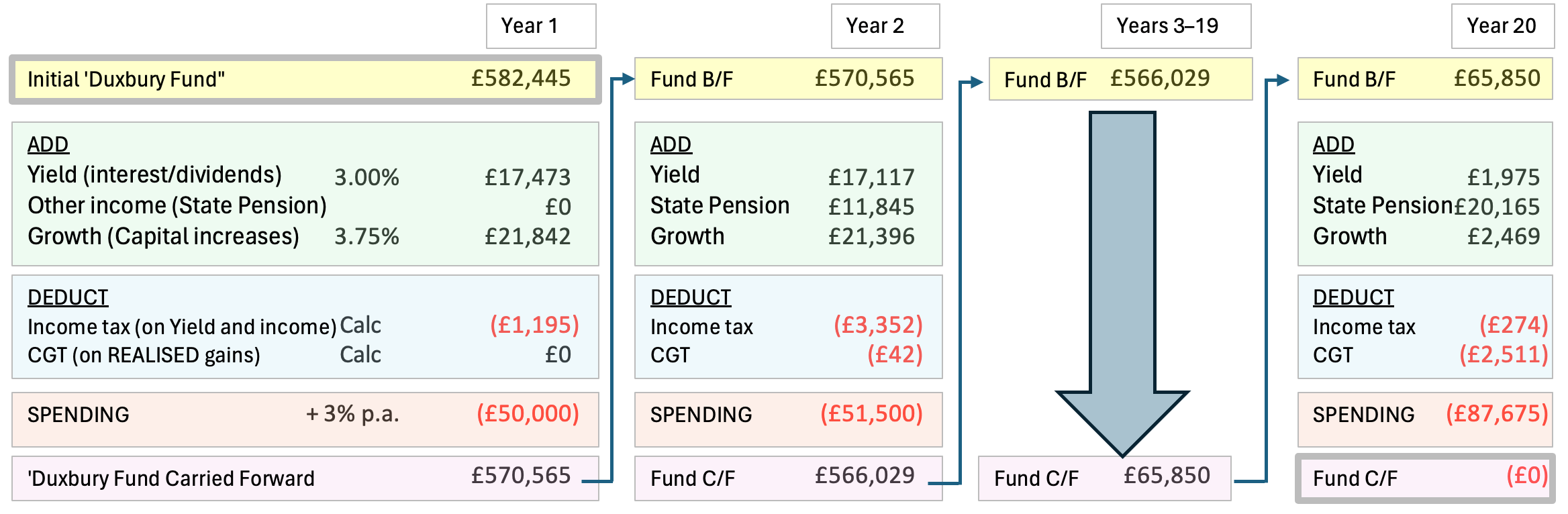
94. This very inexact example shows the first, second and final years of a calculation based on a spending requirement of £50,000 p.a. assuming that a State Pension becomes available in the second year. The tax calculations in this example are illustrative only. The amount carried forward at the end of each year is brought forward to the start of the next. At the end of the chosen period (by default the life expectancy of the payee) the fund is exhausted.
95. The tax calculations are necessarily estimates, based on the current and already announced future rates and allowances, save that beyond any already announced period of freezing such allowances, they are assumed to begin increasing in line with inflation (at 3% p.a.), as is the State Pension. The calculation of Capital Gains Tax (CGT) on realised gains is also necessarily approximated, but under the model all gains made are eventually subject to tax, subject only to the (now much reduced) personal CGT annual allowance.
96. The calculation is always undertaken by starting with a ‘guess’ for the figure at the top left (£582,445 in this example), and the guess is repeatedly refined (‘iterated’) until the figure in the bottom right is, as in this example, £0.
The algorithm – is it fit for purpose?
97. In a wide range of accounting and statistical applications derivative iterative calculations haven proven their worth as an aid to understanding values. For example, in Discounted Cash Flow valuations with which many family law practitioners will be familiar in the context of private companies, and projecting or calculating returns on investments more generally, including calculating Internal Rates of Return on investments and projecting potential ‘carried interest’ or other performance related returns.
98. Such calculations, albeit using different underlying assumptions reflecting the difference between an injured person’s empirical need for continuing care and a divorced spouse’s subjectively assessed reasonable requirements to maintain a given lifestyle, also underlie the Ogden Tables used in personal injury cases.
99. The members of the Working Party are unanimous in our view that the essential algorithm underlying the Duxbury calculation is arithmetically sound, subject to (a) the appropriateness of the underlying assumptions and (b) a proper understanding of what the Duxbury calculation aims to achieve.
Are the assumptions appropriate?
Real returns and inflation
100. It is convenient to take the first three ‘key assumptions’ together. By way of recap they are:
100.1. a uniform income yield of 3% p.a. (1.5% in the first year);
100.2. a uniform rate of capital growth of 3.75% p.a.;
100.3. a uniform rate of inflation at 3% p.a.
101. Together those produce a ‘real’ or ‘inflation adjusted’ assumption of investment return of around 3.75% p.a. over the period of the calculation. The concessionary yield rate of 1.5% in the first year is intended to reflect the inevitable delay in compiling an overall balanced portfolio. This is a crude and somewhat simplistic approach which could be open to criticism as being either too ‘generous’ or too ‘mean’ but it has the virtue of simplicity and only a modest impact on overall outcomes.
102. We have obtained data and analysis from Dimensional Fund Advisors18 for the period 1 January 1990 to 30 November 2023, examining all periods of 15, 20, 25 and 30 years during that 34-year period (i.e. covering returns affected by supposedly ‘black swan’ events of the recent past including the Global Financial Crisis of 2008, the Brexit Referendum in 2016, Covid-19 in 2020/21 and the ‘mini-budget’ of the Truss-Kwarteng administration). The analysis is summarised in this table, which shows ‘real’ rates of return based on an assumed investment portfolio of either 50:50 equities and bonds, or 60:40 equities and bonds:

103. Those figures show that over the relatively recent past, some investors would have achieved more than the 3.75% assumed real return, while others would have achieved somewhat less. Timing is everything with investment, and a claimant who received a Duxbury based award in (say) 1999 – immediately prior to the bursting of the so-called dot.com bubble – would have achieved relatively disappointing returns compared to someone who received their award in say 2010 – immediately after the worst impacts of the Global Financial Crisis had been absorbed. This is a natural and well-understood phenomenon in the investment world. Equally obviously these figures are of average returns and individual investors will have achieved better or worse outcomes depending on the investment choices that they made, and the timing of those choices.
104. In contrast, a comparison with average returns for the same periods from 1915 to 2022 (which includes two World Wars, the Three-Day-Week of 1973/74, the miners’ strike of 1984/85 and numerous other market distorting events) show that the more recent returns referred to above have been modern-historically anomalous:19

105. This in turn begs a question, which we cannot answer, which is whether the most recent investment experience represents a ‘new norm’ or a deviation from the longer-term realities of the markets which will in due course be corrected.20
106. We acknowledge and agree that most Duxbury recipients will have little or no prior investment experience, and their instincts will usually be for security rather than return maximisation, so their actual risk profile will be cautious to very cautious. However, security and caution come at a cost, and the issue is whether that cost should be borne by the payee or the payer in the Duxbury assumptions. To some extent this ‘issue’ is one of education and explanation by financial advisers, who need to be able to justify their investment advice (and the cost of it) in a way which makes it acceptable to the Duxbury fund recipient.
107. We have considered whether it is fair and reasonable to assume that the recipient of a Duxbury based award would or should invest that fund in a mixed portfolio of equities and bonds, and in what proportions, and concluded that the above figures represent a fair band, even if the reality is that such funds are perhaps more likely to be invested more cautiously, and therefore with potentially lower returns. The individual risk profile of the payee – i.e. seeking more rather than less security, in return for the likelihood of lesser rather than greater investment returns – should, we think, not be relevant to the computation of the fair sum to compensate for the forgoing of a periodical payments order. It is not unreasonable to assume that in many potential ‘Duxbury’ cases the ability of the payer to satisfy such an award has depended on their willingness to take entrepreneurial risks and have their own exposure to the vagaries of the markets. We do not consider it appropriate to regard a cautious (or very cautious) investment strategy in an individual case as a reason to adopt lower than reasonably achievable investment returns.
108. That does leave a question about the weighting appropriate as between the more recent figures and those achievable historically. Plainly the more recent figures deserve greater weight as a guide to what might happen in the immediate future, but not in our view to the exclusion of any weight being attributed to the longer-term history. Thus, notwithstanding the shortfall that will have been experienced, on average, by Duxbury fund payees who received their awards more than 15 but less than 25 years ago, we consider that the overall weight of the data supports the continued reasonableness of assumed average real returns of at least the 3.75% p.a. currently assumed, and arguably somewhat higher returns.
109. While those figures broadly support the status quo in terms of overall real investment return assumed there are two important caveats:
109.1. the above figures do not take account of investment management costs, whereas the original assumptions made by Mr Lawrence in 1985 were for returns net of the (then lower) cost of managing the funds; and
109.2. because inflation also affects the other parts of the calculation, including taxation reliefs and allowances and, most importantly, spending, it is necessary also to consider inflation separately as well as part of the real rate of return.
Inflation
110. It would be unusual for a Duxbury fund recipient also to be responsible for funding a mortgage,21 which means that the more appropriate measure of inflation for the purposes of these calculations is the Consumer Prices Index (CPI) rather than the mortgage inclusive Retail Prices Index (RPI).
111. The CPI in July 2024 stood at 171.3:
111.1. 15 years earlier in July 2009 it stood at 110.9 – an overall difference over 15 years of 54.46%, or 2.94% p.a. almost exactly the 3% figure assumed in Duxbury.
111.2. Over 20 years, 25 years and 30 years the CPI measure of inflation has been 2.84%, 2.52% and 2.42% respectively – all of which are lower than the figure assumed in the Duxbury calculation.
112. That inflation (as measured by the CPI) has consistently undershot the assumption made in Duxbury of 3% is a factor which has been favourable to payees, since the assumption has included that their spending requirement would increase annually at a rate greater than inflation. Conversely, but much less significantly, it has also assumed that tax bands and allowances would increase more than they have in fact done.
113. Broadly, therefore, it can be seen that subject to management charges (discussed below) average real returns of a balanced portfolio have approached (and in some cases exceeded) the assumptions, and – at least as measured by the CPI – inflation in relation to expenditure has lagged behind the assumed rate. Overall, although the assumptions may have been marginally more favourable to payees rather than payers, they continue in our view to represent a fair estimate, insofar as such can be made based on historic figures, for deployment in future calculations.
Taxation
114. The next assumption is that of a consistent regime of taxation – with bands/allowances increasing in line with inflation (save that allowances are assumed to be frozen until April 2026 as announced in 2021 by then Chancellor Rishi Sunak and not altered by any of the several successive Chancellors).
115. This assumption is both necessarily simplistic and knowingly wrong. Rates of taxation, and the overall tax ‘take’ vary considerably over time and in both directions. In the most recent past the trend has been unmistakeably upwards overall, although – subject to the imminently forthcoming budget – the headline rates for income tax (including on dividends) and CGT have been relatively stable in the recent past.
116. Changes to National Insurance, Corporation Tax and VAT have little, and usually no, impact on the Duxbury calculation, and most other indirect taxes are captured in the computation of the CPI measure of inflation.
117. However, the freezing of bands and allowances leading to so-called ‘fiscal drag’ has resulted in a higher overall tax burden on recipients of Duxbury based awards than assumed at the time they were computed.
118. Although the freezing of the bands and allowances for income tax will have had some impact on the real-life working out of the tax for Duxbury fund recipients, it is the reduction in the tax-free allowance for Capital Gains and the reduction in the tax-free allowance for Dividend income,22 which will have had most impact in practice. Those changes are, of course, accounted for in the Duxbury model looking forward, but the assumptions made in earlier calculations have been falsified to the detriment of the cohort of payees.
119. There is, at the time of writing, considerable media speculation that the new Labour Government is likely to increase the headline rate of taxation on Capital Gains – perhaps to as much as the corresponding rates of income tax as previous Labour Governments have done. If implemented, such a change would be taken into account for future Duxbury calculations, but those whose awards were computed at a time of a more benign regime will have lost out, just as those who had awards calculated at higher rates prevailing under previous Governments benefited when rates of taxation were later reduced.
120. The uncertainty as to the impact of tax is to some extent, and in some cases no doubt completely, off-set by the absence in the Duxbury calculation of any assumptions that recipient investors will take steps to mitigate tax on their investment returns. If nothing else, even the most inadequate of financial advisers would recommend that the maximum subscription be made each year to ISAs, removing all yield and capital gain from the ambit of tax. The assumptions include that a significant proportion of the fund will be invested in equities, the income from which is taxed at preferential dividend rates, significantly lower than earned income or interest income, but the tax calculation in Duxbury has never descended to the level of precision by seeking to allow for this beneficial rate of tax. Other strategies, for example in relation to Capital Gains on Government Bonds, could serve to shelter other returns. In short, subject to the caveats above about the constantly shifting burden of tax, Duxbury has historically taken a pessimistic view of tax, and in that regard has significantly favoured payees.
121. Taking that rough with the smooth, while at the same time seeking not to over-complicate what is already a multi-faceted computation, we consider that the present approach of adopting the current bands and allowances, and inflating them by the same inflation factor as is used for expenditure save where there has been a pre-announced freeze or other change (in which case the announcement is assumed to end up being implemented) is a fair and reasonable assumption to continue to make, albeit one acknowledged to favour payees.
A constant level of drawdown in real terms
122. It is the essence of the Duxbury calculation when presented in tabular form (i.e. as per the Table in At A Glance) that the assumed rate of required funding remains constant, in real terms, for the whole of the recipient’s remaining life expectancy.
123. Leaving aside the question to which we turn below about the appropriateness of the whole-of-life expectancy assumption, it is more or less obvious that no one will ever, in practice, have a constant and unaltered spending requirement for the rest of their lives or, indeed, over any appreciable period. Life does not work like that. What may appear to be desirable or even necessary items of expenditure for a person in their 50s or 60s, may be quite undesirable and certainly unnecessary when they are in their 70s let alone their 80s. Of course, as items fall away they may well, indeed almost certainly will, be replaced by other items of expenditure the cost of which need bear no relation at all to the items of expenditure which they replace.
124. Certainly since 1995 and the decision of Thorpe J in F v F (Ancillary Relief: Substantial Assets) [1995] 2 FLR 45 there has been awareness, at least in ‘big money’ cases, that levels of expenditure are likely, in real terms, to reduce rather than increase in what he described as ‘the years of dower’ beyond the period of the ‘flood’ of an expensive lifestyle.
125. It is a societal norm – and not only in the UK – that older people, and certainly those beyond retirement age, will tend to have less available to spend than younger people at the height of their earning power (in the case of bread winners) and usually the height of their domestic obligations (in the case of home makers). Accordingly, retirement income and expenditure are normally expected to be lower than pre-retirement income and expenditure. To some extent this is facilitated by the reliefs and ‘concessions’ available to older people, and – of course – the receipt of State Benefits in the form of pensions on an entitlement rather than means-tested basis.
126. More sophisticated Duxbury calculators (such as Capitalise by Class Legal) allow for the tailoring of expenditure requirements, in both directions, but in a two-dimensional tabular form as in At A Glance, the assumption of a constant real rate of drawing is in our view favourable to recipients/payees in the majority of cases.
Churn
127. The calculation assumes a consistent rate of ‘churn’ (the realisation of capital gains other than to fund expenditure) equal to 3% p.a. This is a sophistication to the calculation to reflect the ‘real world’ fact that sometimes gains will be realised other than to fund expenditure, which will serve to increase by bringing it forward, the taxation of such gains.
128. We have not considered it necessary to examine whether this assumption, which has never been the subject of criticism or even discussion in any of the many articles written about Duxbury over the years, should be revisited.
Life expectancy
129. Duxbury, certainly as published hitherto in At A Glance, has always assumed that the recipient will survive for precisely the expected average of their contemporaries.
130. Life expectancy is the age by which 50% of the population of a particular age can be expected to have died.
131. On one level this is a necessary and knowing simplification. It would plainly be impracticable for even bespoke Duxbury calculations fairly to be undertaken on a case-by-case individualised assessment of life expectancy. Even taking account of family history, personal medical history and more or less hazardous lifestyle choices, the art of predicting how long an individual is likely to live, other than by reference to their statistical and actuarial life expectancy is a fool’s errand – rightly eschewed even in the small number of cases where it could be confidently asserted that a life expectancy was greater or, more usually, lesser than the actuarial table would dictate.
132. Moreover, there is no such thing as a single ‘life expectancy’. Rather there are various different projections from various bodies, most notably (in the UK) by the Government Actuaries Department based on data from the Office for National Statistics (ONS). At any one time there will be several different tables available of estimated life expectancies of different cohorts based on social class, membership of pension schemes and a variety of other factors. The variance between such datasets may be great or small for a person of a specific age.
133. Were it not for our main conclusion (as discussed below) relating to the inappropriateness of the assumption of whole-of-life computations, we might have sought outside assistance from the Government Actuary as to whether the current selection of the ONS20 whole UK national projections, as used in the computations in At A Glance, is appropriate, although we have no reason to consider that it is not. A choice has to be made which is of general application to the population as a whole, and ONS20 seems to us to be as rational a choice as any other.
134. However, we are unanimous in our view that while whole-of-life is a permissible, and in some cases appropriate, basis for a Duxbury calculation, it should not, in the light of societal changes and in particular the near extinction of the whole-of-life periodical payments order, be as hitherto the default.
135. Rather, we are of the view that the process should become one of two stages – as it presently is in a continuing periodical payments case:
135.1. What is the appropriate level of financial support to be made for the benefit of the payee by the payer?; and
135.2. What is the appropriate duration for such support to be provided?
136. Considering those two stages separately will throw up a figure based on the number of years in the second stage, which may be quite different from the actuarial life expectancy. The figure may be affordable by the payer (in which case there can be a clean break on payment of the appropriate figure) or it may not be affordable in which case either a hybrid award (periodical payments for a period followed by a smaller lump sum) or a continuing periodical payments award would follow.
137. In considering the quantum and/or duration of the required support the court would be able to take into account whether the recipient was entitled to a State Pension (rather than the current default that such entitlement exists), and the impact of any pension sharing award or pre-existing pension held by the recipient. Pension sharing was not available in 1985 when Duxbury was decided.
138. There will, of course, continue to be cases in which whole-of-life provision is appropriate, but we cannot see why it should be the default assumption. That assumption was perhaps fairly made under the old, pre-White, regime of paternalistic protection by the court of otherwise financially disadvantaged claimants. But in the modern era, and regardless of proposed reform to the law of financial remedies limiting periodical payments to a relatively short timeframe, it appears to us to be an anachronistic legacy inconsistent with the development of the law more generally.
139. To put it another way, if in a case where capital has been shared, but where (per Waggott [2018] EWCA Civ 727) income is not to be shared but is to be allocated by way of needs-based provision as periodical payments subject to the enjoinder for the court to consider ‘whether it would be appropriate to require those payment to be made … only for such term as would … be sufficient to enable the party in whose favour the order is made to adjust without undue hardship …’ then why should a payment in substitution for such a periodical payments order be calculated on a whole-of-life basis by default?
140. We therefore propose a new presentation of the now familiar Duxbury calculation table, based on a number of years for a fixed annual spend. The table would be age and gender neutral, and not include the hitherto built-in discount for an assumed full State Pension. The existence or not of such an entitlement would be factored into the duration of the provision (or perhaps the quantum) rather than hard-baked into the calculation. The differences in life expectancies between men and women could be, but does not have to be in every case, reflected in the selection of the duration element of the award. This feeds directly into the next assumption to be discussed.
The full State Pension
141. The Duxbury calculation has always assumed that the recipient is or will become entitled to a ‘full’ State Pension at their current pension age.
142. As the Women Against State Pension Inequality (WASPI) campaign has made widely known, that assumption – even in the case of those women who had built up the necessary entitlement to receive such a pension – has not necessarily held good as the pension age has progressively moved backwards from 60 to a presently fixed, but likely to be further extended, age of 68.
143. Moreover, while in 1985 almost all divorcing wives would have been entitled to a State Pension based on their husband’s National Insurance contributions, such entitlement now accrues only based on their own contributions.
144. Although it is also true that a large proportion of the adult population, including married women and mothers, are now in employment outside the home and likely to be making the necessary National Insurance contributions for at least the majority of the necessary contribution period, there will still be a sizeable number of claimants in financial remedy proceedings who do not have any State Pension entitlement, or less than the full amount.
145. We consider that it is relatively easy when considering the duration of a proposed periodical payments or capitalised (Duxbury) award to take account of the existence or not of such entitlement, and particularly so when coupled with a pension sharing award or pre-existing pension entitlement, to arrive at a fair outcome. On the other hand, we consider that it was and is more difficult for a court or legal adviser to consider what increase should be made to a conventionally ascertained Duxbury award, based on a two-dimensional table of the kind appearing in At A Glance, to reflect any shortfall in the individual’s State Pension entitlement. It is one thing to know that it should increase the award, but quite another to work out by how much.
146. Removing the State Pension element from the illustration at paragraph 93 above results in an increase (for a calculation undertaken over 20 years) in the fund required from £582,445 to £716,623, an increase of about £134,000 or about 23%. This divergence is towards the top of the range previously identified in At A Glance for the adjustment necessary when a State Pension is not, in fact, going to be received:
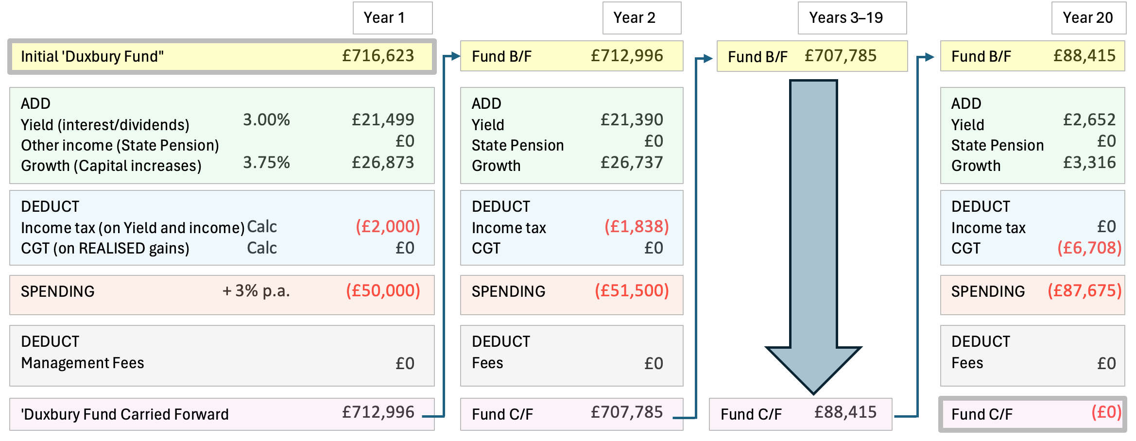
Pension inflation
147. The Duxbury assumption has been that the State Pension will increase at the assumed rate of inflation (rather than the probably higher rates of wages in general or 2.5% as guaranteed under the ‘triple lock’).
148. Given our conclusion as to the appropriate mechanism as discussed in the previous section, this assumption is rather less significant under our proposed model than under the existing model.
149. It is an assumption which has been extremely favourable to payees (except a small class of the WASPI age-group), to the cost of payers. State Pension inflation has outstripped inflation over the last 15, 20, 25 or 30 years – even allowing for the later date of commencement for some recipients. Particularly for those entitled to the ‘new’ State Pension (i.e. men born after 5 April 1951 and women born after 5 April 1953) pension inflation has been substantial.
150. The effect of the ‘triple lock’ is that in reality pension inflation will continue to outstrip general inflation.
Pension age
151. As already mentioned, the assumption made in Duxbury has traditionally been that the age from which the State Pension is payable will not alter in the meantime. Like all of the assumptions, this is a knowingly false assumption, made because some assumption has to be made.
152. Pre-announced changes are already built into the calculation.
153. Insofar as, contrary to our proposal, pension entitlement continues to be part of the algorithm, we consider that it is fair to assume that the existing and pre-announced changes to pension ages will apply to the individual under consideration. Naturally, the younger the individual the more likely it is that this assumption, and any or all of the others, will be falsified by events unfolding over the ensuing decades.
154. To the extent that old Duxbury awards were based on an assumed State Pension age which has been falsified by the progressive increases in that age, that will have been to the detriment of payees and the benefit of payers. In practice, such changes were announced and taken into account by the Duxbury calculation many years (and in some cases decades) earlier, so whatever may have been the state of ignorance of the WASPI complainants, any Duxbury payees in that rank will probably not have been disadvantaged.
Conclusion on the assumptions
155. Subject only to the questions of (i) fund management charges (ii) the continued reliance on a default of whole-of-life support and (iii) the default inclusion of a full State Pension, we therefore conclude that the ‘assumptions’ continue to represent a reasonable basis for the undertaking of capitalisation calculations.
156. While there will be those cases – we anticipate very much a minority – in which the facts, including for example the security of the paying party’s financial position (the super-rich) or the age of the claimant (already at or close to retirement age) might justify the court adopting a whole life approach to capitalisation, we are collectively somewhat mystified that this has been the tacit default in almost all reported ‘Duxbury’ cases over the last three decades.
Management charges
157. Our enquiries have revealed that charges, including both fees for advice and management and the costs associated with dealings, might typically be in the order of 1.5% p.a. on a medium sized portfolio, but somewhat less on a larger portfolio.
158. There appears to be very considerable variance in relation to fees including at least the following factors:
158.1. some fees are calculated on the basis of the funds under management or in respect of which advice is given, while others or other providers, charge fixed or pre-agreed fees;
158.2. some providers have published stepped rates, with a lower percentage charge for larger portfolios, while others publish only flat rates;
158.3. some providers are amenable to individual negotiation on fees, perhaps particularly for larger portfolios and will ‘compete on price’;
158.4. some investors (payees) will be willing to engage in negotiation and/or be prepared to change providers in search of a better deal, while others, through inertia, or loyalty, or lack of knowledge, will remain with the same advisers and the same platforms regardless of price; and
158.5. in periods of high returns, as have been enjoyed in the immediate past, investors are willing to tolerate levels of fees which might be less palatable during periods of lower returns.
159. Those charges are not in general allowable against tax on yield or capital gains.
160. Historically, as stated in ‘Reflections on Duxbury’ in the 1995 edition of At A Glance (see paragraph 17 above), and as recently accepted by Moor J in his judgment in MN v AN [2023] EWHC 613 (Fam), the ‘assumptions’ in Duxbury have been inclusive of management charges. We are concerned that the data does not necessarily support the average achievability of such returns after charges.
161. The impact of such charges (say 1.5%) on the real rates of return illustrated at paragraphs 102 and 104 above is obvious and potentially significant.
162. The average real rate of return of the 50:50 (equities to bonds) portfolio would be reduced to about 1.62%, and for the 60:40 portfolio to about 2.17% if relying on the historic data only since 1990.
163. Taking the longer view relying on data over the period since 1915 would reveal long-term real returns net of charges of 1.5% p.a. to be 3.77% (50:50 portfolio) or 4.18% (60:40 portfolio).
164. The former – and arguably the more relevant data being the most recent – shows a sharp divergence from the assumptions presently adopted in the Duxbury calculation, whereas the latter tends to show that the present assumptions may be conservative.
165. We have not found it easy to reach any firm conclusions on how, if at all, the Duxbury calculation should be adjusted to reflect the impact of management charges and fees.
166. A purist approach – seeking to attribute arithmetical justification for every variable and to further complicate the computation – holds a certain appeal, and we have considered whether an additional allowance should be introduced into the algorithm to deduct such charges after computation of the annual tax charge.
167. Some of us have concluded that the overall algorithm is already quite materially slanted in favour of the majority of claimants/recipients for the reasons which we have explained above relating to the exclusion of the factors would which be likely to have led to a reduction or termination of the periodical payments order had such an order been made rather than capitalised. This is true whether the current default of whole-of-life is retained or replaced, as we recommend, with the two-stage approach in which the amount and duration are assessed separately as part of the capitalisation calculation, although perhaps less so if the reforms we propose were to be adopted.
168. We acknowledge that this would result – as Duxbury always has – in winners and losers amongst the recipients. Those who are long lived and remain single will, as now, be at risk of being underpaid by reference to the fund necessary to enable them to live at the given rate for the rest of their lives. They are the losers. Those who are either short-lived (dying before their fund is exhausted despite being drawn as anticipated) or who remarry or otherwise adjust their living arrangements so as to end their entitlement to dependence on the payer are the ‘winners’. To the winners must also be added the payees in those cases in which the fortunes (including health) of the payer take a downward turn so that the periodical payments order, had one been made and not capitalised, would have been reduced or terminated as a result of the change in their circumstances.
169. Some of us consider that the potential investment return shortfall, if indeed there is such a shortfall, whether as a result of macro-economic factors, investment decisions or fund management charges, is a fair risk for the cohort of recipients to be required to assume to balance the advantage that the same cohort has by reason of the non-variability of the capitalised award.
170. However, others of us consider that the impact of management charges is a separate ‘assumption’ which should be baked into the computation. If the computation is to be based on investment returns which can realistically only be achieved with the assistance of professional fund managers, allowance must be made for the deductions from the fund to meet their costs.
171. Establishing what those costs are likely to be is problematic for the reasons just given. Different platforms and different advisers have different charging rates. We have obtained anecdotal and informal soundings from various potential managers and advisers, and the range is wide and the pattern inconsistent.
172. Aware that this is something of a compromise our conclusion has coalesced around making some allowance in the basic computation, by allowing for a deduction while leaving the other underlying assumptions unchanged. We have opted for a graduated charge, with funds under £1m suffering 1% p.a., and funds over £1m suffering 1% on £1m and 0.5% on the value of the funds in excess of £1m. Thus, a fund of £3m would suffer annual charges of £1m x 1% + £2m x 0.5% = £20,000 or 0.67% overall. We propose that as with tax allowances, the £1m band is ‘inflated’ each year in accordance with the general rate of inflation adopted. By the end of any fund the rate will be 1% as the amount in the fund dwindles below the inflated first ceiling of £1m in real terms. We consider that this compromise effectively allocates some of the likely actual charges to the payee and some to the payer. In any individual case that is likely to strike a fair balance. Requiring the payee to shoulder some of the charges is an additional counterbalance to a powerful but unquantifiable imponderable operating in their favour namely that they do not have to repay any part of the Duxbury fund if they remarry or re-partner before the expiration of the assumed term or if the payer dies in that period.
173. There may be individual cases in which a party might be able successfully to argue for a bespoke calculation based on different assumptions, including in relation to management charges, but for the purposes of the vast majority of cases in which a two-dimensional Duxbury table is utilised as the guideline for the appropriate figure, we commend the compromise in the previous paragraph.
174. Reworking the calculation illustrated at paragraph 146 above by allowing an additional deduction for management charges increases the initial fund required to £789,484 (an increase of c. £207,000 (or +35.5%) on the original requirement calculated in accordance with the current assumptions illustrated at paragraph 93 above):
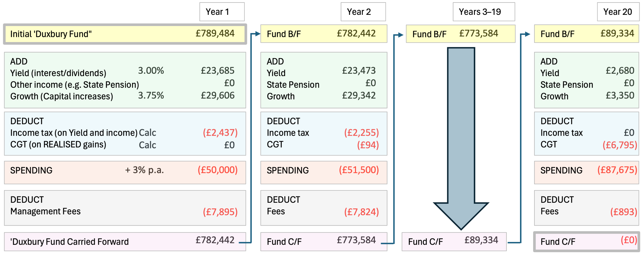
175. However, we would not envisage that the ‘new’ Duxbury Calculation for a payee would be undertaken without regard to whether the payee did in fact have an entitlement to a State Pension.
176. The example we have been using is based on a female payee aged 66 or 67 at the commencement of the period. For reasons we have explained above, we anticipate that a court approaching such a case would assess the spending need first, and in doing so would be able to consider to what extent that might be met by a pension if the payee had any such pension (whether State Pension or as the result of a pension sharing order or from an occupational or otherwise self-funded pension) before fixing the amount of spending to be met from the capitalised part of the award. The court would then consider over what period that financial support should be provided – which might be based on life expectancy but, more usually we suggest, some lesser period.
177. In our example, if the court was aware that the payee would soon become entitled to a full State Pension of (say) £11,500 p.a. it might assess the spending requirement at perhaps £50,000 less 80% of £11,500 (to allow for the tax on the pension) = £40,800. It might also assess that the appropriate duration of the award was – in view of the payee’s age and despite our overall recommendation to move away from whole of life awards, to be taken as their life expectancy of 20 years. It would thereby arrive at a figure of about £638,000 – or around £56,000 (10%) more than under the current assumptions. This is the effect of allowing separately for the management charges.
178. But for a much younger payee, say in their late 40s or early 50s, the court might entirely disregard any entitlement to a State Pension, allow for a full ‘budget’, and management charges but at the second stage limit the term of the financial provision to, perhaps the number of years of the payer’s remaining working life prior to their State Pension age. That would, for younger payees, potentially significantly reduce the overall term over which the sum was calculated, eliminating or mitigating the so-called Duxbury paradox (the younger the claimant the higher the award and vice versa). We discuss this further in the section ‘The whole-of-life assumption’ below.
Bespoke calculations
179. Consistency and predictability militate strongly against encouraging or even permitting bespoke calculations in relation to ‘assumptions’ in individual cases in the absence of some special factor taking the case out of the usual run. Obviously bespoke calculations dealing with earnings, changes in spending requirement, capital injections and things of that sort, which do not depend on adjusting the ‘assumptions’ are often required and helpful.
180. It would be time and costs wasteful to have, or encourage, bespoke calculations in standard cases, and the easy availability of published tables from which guideline figures can be ascertained should, in our view, be sufficient in nearly all cases.
181. While the previously published tables – including, and most notably, those in At A Glance – have stood the test of time, as we have mentioned above we consider that the time has come for a revised presentation to be made available for use in our proposed two-stage computation abandoning the whole-of-life default.
182. Even if bespoke calculations were to be permitted in an individual case, we consider that a judge accepting evidence based on the subjective characteristics of the proposed payee (for example the longevity of their parents) would be entering dangerous and uncharted waters. For one thing the admission of such evidence would be difficult to distinguish from the admission of evidence tending to show that the payee had a shorter than statistically average life expectancy, by reason of a pre-existing condition or habit (such as alcoholism or smoking) or family history. For another, such evidence would have to be scientifically robust23 and would amount to expert evidence requiring the court’s permission to adduce and meeting the necessity threshold test. It is also difficult to see how a judge would be able to avoid case specific evidence about prospects for remarriage or cohabitation. We perceive this to be a slippery slope towards unpredictability and inconsistency which should be discouraged.
The whole-of-life assumption
183. At the risk of unwelcome repetition, we return to our main conclusion which is that while the algorithm as a whole, and the underlying assumptions taken as a whole, remain viable and reasonable, we are troubled by the default of whole-of-life provision.
184. Duxbury has for many years come with a warning against its deployment in cases where, by reason of the advanced age of the payee, the life expectancy is less than about 15 years. This is for the very obvious reason that once life expectancy is that short it becomes possible to outlive it by a very substantial margin in proportionate terms. A woman of 78 years with a life expectancy of 11.5 years, might well live to 101 – more than double her expectancy. A woman of 58 with a life expectancy of 29 years has almost no chance of living to 116.
185. We consider, in the surely very rare case where an assessment of the needs of a claimant over (about) 75 is undertaken, the consequences of the unfolding facts differing from the initial assumptions could be so severe, that a Duxbury capitalisation would not be appropriate. In such a case the purchase of an annuity, or the fixing of the award by reference to the cost of doing so, may well be apt. An alternative may be to adopt a Duxbury calculation utilising a longer-than-life-expectancy basis, perhaps with the ‘balance’ held on trust to revert to the payer on the payee’s death provided the payer was the survivor, or to their estate if they were not. Such outlier cases should not lead to the tail wagging the dog of the great majority of cases.
186. The problem of the whole-of-life default is particularly acute in relation to younger payees – i.e. those with an actuarial life expectancy of more than about 30 years – i.e. men under about 54 and women under about 58 years of age, and spectacularly so for those with a life expectancy greater than 40 years (men under 45 and women under 47), since the practical likelihood a periodical payments order remaining in payment for such periods is self-evidently slim to non-existent.
187. It is not for us to devise new defaults, and any proposal for which would need to be fully argued and the subject of consultation if not judicial determination. It may be that future legislative reform in relation to periodical payments will render this discussion moot, but for the moment we recommend that parties and courts might consider arguably more generous quantum, perhaps (in an appropriate case where pension assets are insufficient to meet relationship-generated retirement need and resources are sufficient to render a stockpiling element fair) to include an element of ‘stock piling’24 coupled with less than whole-of-life durations, taking into account factors such as the anticipated working life of the payer, the presence or absence and duration of the remaining domestic contributions of the payee and the length of the relationship relative to ages of the parties, as factors which might lengthen or curtail the duration. This would enable the known or anticipated pension position of the payee to be taken into account in assessing both quantum and duration of the dependency to be capitalised.
188. To this end we have created and placed in Appendix 5 a ‘new’ Duxbury table which, with interpolation, enables the easy computation of a capitalisation award for a wide variety of plausible amounts and durations, but would force the separate consideration of the latter without the default of whole-of-life.
Education and ‘health’ warnings
189. As we have adverted to above, we perceive that a good deal of the disquiet in relation to past Duxbury awards has arisen from a misunderstanding of what the computation aims to do, and the necessary balance to be struck between payees and payers.
190. In this report we have first addressed the inconsistency that while a joint lives maintenance order is a now an exceedingly rare bird, the whole-of-life Duxbury award has been the court’s almost invariable approach. We have sought to resolve that inconsistency by devising a revised Duxbury table which gives capitalisation figures for various terms (which, of course, could correspond, as before, to the subject’s life expectancy). The figures in the revised table have been calculated using, for the first time, management charges as an additional discrete key assumption.
191. The following points should be included in advice to clients:
191.1. A Duxbury calculation is not designed to identify (and will not achieve) a sum necessary to guarantee a particular level of expenditure and precision of calculation is never achievable. It must be clearly distinguished from a pension which will pay out indefinitely.
191.2. The calculation is based on a range of assumptions as to life expectancy (if that is the term being used); inflation, management charges; rates of income yield and inflation; and tax rates. It may also allow for receipt by the subject of a full State Pension. None of these may be fully accurate for that individual. This should be clearly pointed out to clients.
191.3. Financial planners/advisers often make the point that a cautious investor payee will not have the appetite for risk that will achieve the illustrated income. In contrast, the payer, perhaps a more adventurous investor, may argue that a higher return could be achieved. This is the key point with Duxbury. It is a tried and tested, judicially accepted and endorsed, illustration giving a capital figure for the sum required to meet the recipient’s income needs over a specified term. But, like Heather Mills,25 the recipient might remarry within that term. Had the payee been in receipt of periodical payments they would have terminated automatically. So, in that scenario the payee has ‘beaten’ Duxbury. Similarly, the payer could lose their job and successfully apply for a downwards variation or discharge of a joint-lives maintenance order. In that case the payee of a Duxbury fund has beaten it again. Conversely, the payee may invest more cautiously, or use more expensive advisors, or live for longer than the actuarial age. In those scenarios the Duxbury sum will not be enough, and it will be exhausted before the expiration of the utilised term, or more likely the payee will have had to rein in their expenditure to prevent that from happening. The mathematical initial number will not turn out to be the right number in the events that unfold – that is the only guarantee. As Ward J stated in B v B [1990] 1 FLR 20 ‘The only certainty is that it will not happen as we have predicted’. And Baroness Hale in Simon v Helmot [2012] UKPC 5 at [72]: ‘However, Duxbury calculations do suffer from the uncertainties of prediction. Nothing will in fact turn out exactly as it is predicted to turn out, whether in family law or in personal injuries law.’
191.4. Financial advice could be sought before making proposals or reaching an agreement, so that the payee might have a financial adviser’s perspective (but which is still only an estimate) on what income the payee might expect to receive from a given capital sum using different assumptions. But the payee should be made aware that it is unlikely that arguments proposing the use of different assumptions (let alone a different method of calculation) will be accepted. Clients should be told that while the calculation is a ‘tool not a rule’, experience shows that it is tends to be closer to the latter than the former.
The Duxbury Working Party
Michael Allum
Simon Bruce
Sarah Hoskinson
Lewis Marks KC (Chair),
Sir Nicholas Mostyn
Joseph Rainer
Mary Waring
Appendix 1: Short biographies of the members of the reconstituted Duxbury Working Party
Michael Allum
Michael is a solicitor at The International Family Law Group LLP. He specialises in financial issues which arise on relationship breakdown, with a particular focus on cross border and international cases. He is also a member of the Financial Remedies Journal editorial board.
Simon Bruce
Simon Bruce is a solicitor and Partner at Dawson Cornwell LLP. He is also a pro bono lawyer at law clinics in London. Simon has practised for over 41 years.
He’s on this Duxbury Committee as he had the cheek to write a critique on Duxbury more than a decade ago. Simon writes the ‘Thought Leader’ in Family Law. He comes from Lancashire.
Sarah Hoskinson
With over 20 years’ experience in complex financial remedy cases, Sarah is a Partner and Head of Burges Salmon’s Family & Divorce practice. She sits on a number of financial remedy and other technical groups, including the Family Justice Council Financial Remedy Working Party, FJC Working Party on Needs, the Pension Advisory Group (PAG and PAG2) and the IAFL Pensions Committee, which she chairs.
However, it is through her membership of Resolution’s Financial Remedies, Tax and Pensions Committee that she became involved in the Duxbury Working Party in 2023. Her approach to all of the work she has done in these groups, the Duxbury Working Party included, is to focus on relevant and practical education for family lawyers on the technical issues, and how they apply in practice.
Lewis Marks KC (Chair)
Lewis has been a barrister for over 40 years, a QC (now KC) since 2002 and has specialised in financial remedy cases for most of that time. He has appeared in many of the leading cases (including as junior counsel in White in the House of Lords, as leading counsel in the Court of Appeal in Miller and dozens of influential cases at first instance in the High Court and on appeal to the Court of Appeal).
He has been an editor of At A Glance since 1999, and is also a founder editor of the Financial Remedies Practice.
He was an original member of the Duxbury Working Party in 1998 and has authored a number of papers on the subject of Duxbury calculations. He has acted a Chair and convenor of the reconstituted Duxbury Working party. He has no judicial aspirations.
Sir Nicholas Mostyn
Nicholas was a barrister for 30 years specialising in matrimonial finance cases, appearing as a QC in the foundational decisions of the House of Lords in White v White (2000) and Miller v Miller (2006) and of the Supreme Court in Granatino v Radmacher (2010).
He became a High Court judge in 2010 and sat in the Family Division, where he gave many judgments of importance in the financial remedy field.
He was a founder editor of At A Glance in 1992 (now in its 33rd edition) and of Financial Remedies Practice in 2011 (now in its 13th edition) and continues as editor-in-chief of both publications.
He was also a judge of the Court of Protection and of the Administrative Court of the King’s Bench Division of the High Court where he heard many judicial reviews of government decisions. Renowned for his independent, outspoken style, he frequently challenged the received wisdom of the law in favour of justice.
He retired from the Bench in July 2023, three years after being diagnosed with Parkinson’s Disease, since when he has become an acclaimed podcaster. In July 2024 he was awarded a Doctorate of Laws honoris causa by his alma mater Bristol University.
Joe Rainer
Joe is a barrister who specialises in financial remedy cases. He is a (relatively new) editor of At A Glance, a co-author of the fourth edition of Pensions On Divorce: A Practitioner’s Handbook, and a member of the Financial Remedies Journal editorial board and the Pension Advisory Group.
Mary Waring
Mary is a chartered financial planner, chartered accountant and Resolution Accredited Specialist.
She is the founder of Wealth for Women, an award-winning company, specialising in financial advice to women going through divorce, especially those who haven’t been responsible for the finances during their marriage. She supports clients through this particularly challenging time who need trustworthy expertise and guidance. She works with her clients, so they understand the options available to them based on their financial situation and know how to improve their future.
Mary was interested in joining the Duxbury Working Party since her clients are typically non-earning spouses and have been for maybe 25+ years. They are therefore unlikely to become major income earners post-divorce.
Appendix 2: Key assumptions adopted in At A Glance 1992–2025
| Edition | Income yield % | Capital growth % | Inflation % | Real rate of return % | |
| 1992 | 6.00 | 6.00 | 7.00 | 5.00 | |
| 1993 | 5.00 | 4.00 | 4.00 | 5.00 | |
| 1994 | 4.50 | 2.00 | 2.00 | 4.50 | |
| 1995 | 4.25 | 2.00 | 2.00 | 4.25 | |
| 1996 | 4.25 | 3.00 | 3.00 | 4.25 | |
| 1997 | 4.25 | 3.00 | 3.00 | 4.25 | |
| 1998–1999 | 4.25 | 3.00 | 3.00 | 4.25 | |
| 1999–2000 | 3.25 | 4.00 | 3.00 | 4.25 | |
| 2000–2001 | 3.25 | 4.00 | 3.00 | 4.25 | |
| 2001–2002 | 3.25 | 4.00 | 3.00 | 4.25 | |
| 2002–2003 | 3.25 | 4.00 | 3.00 | 4.25 | Note 1 |
| 2002–2003 | 3.00 | 3.75 | 3/00 | 3.75 | Note 1 |
| 2003–2004 | 3.00 | 3.75 | 3.00 | 3.75 | |
| 2004–2005 | 3.00 | 3.75 | 3.00 | 3.75 | |
| 2006–2007 | 3.00 | 3.75 | 3.00 | 3.75 | |
| 2007–2008 | 3.00 | 3.75 | 3.00 | 3.75 | |
| 2008–2009 | 3.00 | 3.75 | 3.00 | 3.75 | |
| 2009–2010 | 3.00 | 3.75 | 3.00 | 3.75 | Note 2 |
| 2010–2011 | 3/00 | 3.75 | 3.00 | 3.75 | Note 3 |
| 2011–2012 | 3.00 | 3.75 | 3.00 | 3.75 | Note 3 |
| 2012–2013 | 3.00 | 3.75 | 3.00 | 3.75 | Note 3 |
| 2013–2014 | 3.00 | 3.75 | 3.00 | 3.75 | Note 3 |
| 2014–2015 | 3.00 | 3.75 | 3.00 | 3.75 | Note 3 |
| 2015–2016 | 3.00 | 3.75 | 3.00 | 3.75 | Note 3 |
| 2016–2017 | 3.00 | 3.75 | 3.00 | 3.75 | Note 3 |
| 2017–2018 | 3.00 | 3.75 | 3.00 | 3.75 | Note 3 |
| 2019–2020 | 3.00 | 3.75 | 3.00 | 3.75 | Note 3 |
| 2020–2021 | 3.00 | 3.75 | 3.00 | 3.75 | Note 3 |
| 2021–2022 | 3.00 | 3.75 | 3.00 | 3.75 | Note 3 |
| 2022–2023 | 3.00 | 3.75 | 3.00 | 3.75 | Note 3 |
| 2024–2025 | 3.00 | 3.75 | 3.00 | 3.75 | Note 3 |
Note 1 – two tables were published: one with a 4.25% RRR, the other with a 3.75% RRR.
Note 2 – income yield for year 1 set at 0% and for year 2 at 1.5%.
Note 3 – income yield in year 1 set at 1.5%.
Appendix 3: A list of the articles which we have considered
- Singer and others, ‘Duxbury – The Future’ [1998] Fam Law 741. (Paper of the Duxbury Working Party: Singer J, Nicholas Mostyn QC, Lewis Marks, Peter Lobbenberg, Timothy Lawrence, Adrian Gallop, Dominic Wreford and Nicola van Lennep)
- Woelke, ‘Is Duxbury the Answer?’ [1999] Fam Law 766
- Mostyn, ‘Is Duxbury the Answer? Yes is the Answer’ [2000] Fam Law 52
- Merron, Baxter and Bates, ‘Is Duxbury Misleading? Yes It Is’ [2001] Fam Law 747
- Marks, ‘Duxbury – The Future? Episode II’ [2002] Fam Law 408
- Gold, ‘Civil way’ 159 NLJ 1030, 17 July 2009
- Phillpotts and Bruce, ‘An Alternative View of Duxbury’ [2010] Fam Law 161
- Marks, ‘An alternative view of Duxbury: A Reply’ [2010] Fam Law 614
- Hitchings, ‘Reconsidering the Duxbury default’ [2021] 33 CFLQ 275
- Allum, Jenkins and Gilbert, ‘Looking back at Duxbury 30 Years On’ [2023] FRJ 11
- The commentary on Duxbury in each edition of At A Glance as listed in Appendix 2
Appendix 4
The indices used to generate the figures in paragraphs 102 and 104 were as follows.
Dimensional used the Bloomberg Aggregate Bond Index for the bond element in each example. The bond element was reduced by 2% held as cash as most platforms require a cash balance to cover upcoming fees. The MSCI All Country World Index was used for the equity element.
For their analysis, Timeline used the Morningstar Global All Cap Target Market Exposure Index for the equity element and the Global Aggregate Bonds Unhedged – Morningstar Global Core Bond index for the bond element.
Appendix 5: Capitalisation in whole thousands of pounds to three significant figures
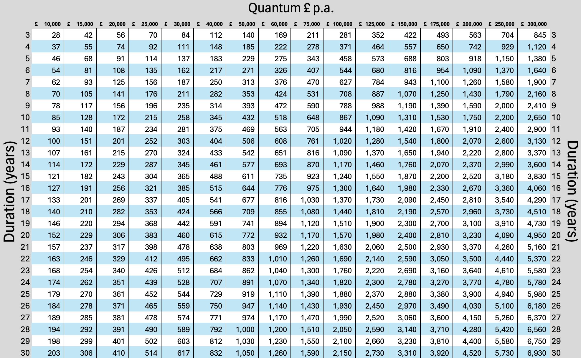
% discount factors
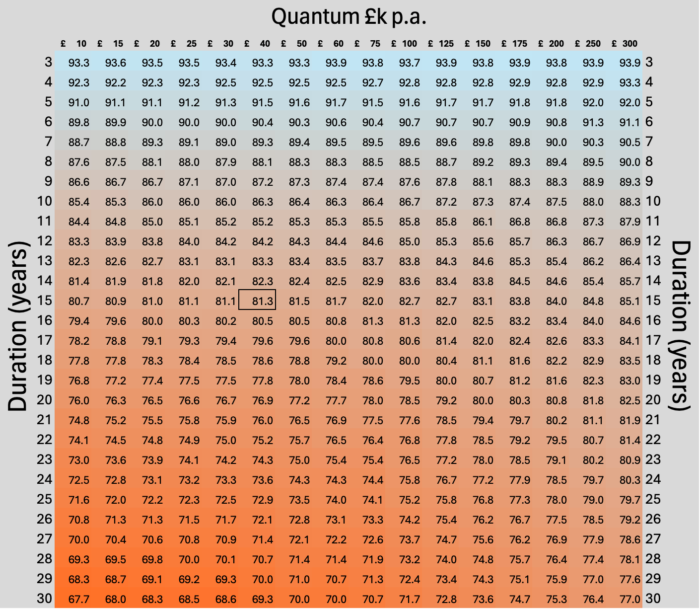
- This version allows for easy interpolation of any number of years or quantum. The figures shown are the overall discount on simply multiplying the quantum by the duration in years.
- For example, £40k x 15 years (bare multiplication gives £600,000).
- The discount factor (shown boxed) is 81.3%.
- 81.3% x £600,000 = £487,800.
- Compare with £488,000 on the detailed table.
- Thus one could interpolate for £45,000 for 15 years by taking an average of 81.3% and 81.5% = 81.4% x £45,000 x 15 = £549,450, say £549,000.
 ©2024 Class Legal classlegal.com